Overview
In this section, we describe the basics of the GELATO model.
How to describe the locations of tracers
The positions of the tracers used in the GELATO are represented using normalized coordinates in the downstream and transverse directions. For example, when boundary-fitted coordinates are used for rivers, as shown in Figure 1 , Non-dimensional coordinates of \(\xi\) in the downstream direction, and \(\eta\) in the transverse direction show the location of the tracers using values between 0 to 1.
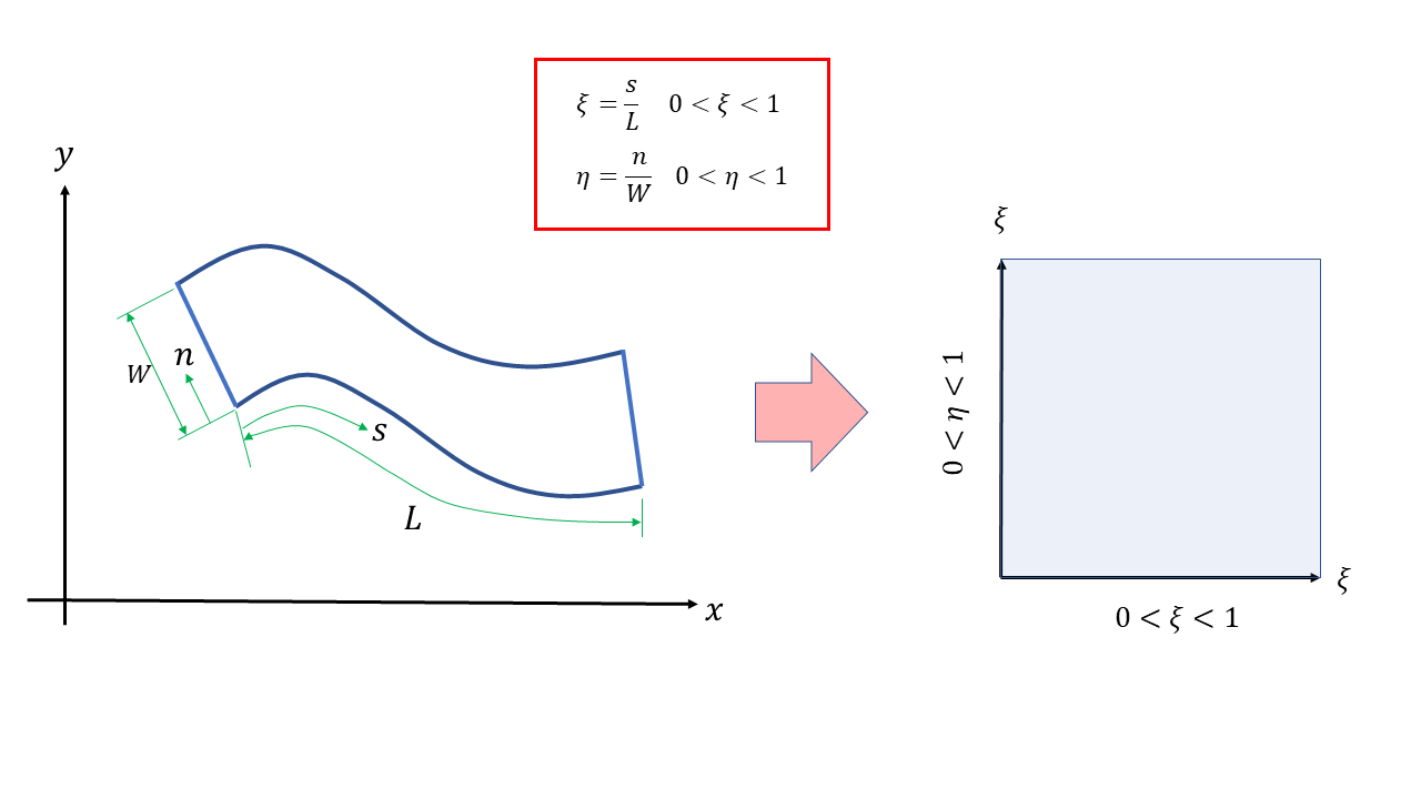
Figure 1 :Non-dimensional description of tracers’ position
Random walk model considering the effect of turbulence
According to Callies (2011), and McDonald and Nelson (2020), the target tracer’s position vector \(\boldsymbol{r}\) is expressed by the following equation
\[\boldsymbol{r}(t+\Delta t) = \boldsymbol{r}(t)+ \boldsymbol{U} \Delta t + \boldsymbol{U}_p \Delta t + \boldsymbol{L}\sqrt{2K\Delta t}\]
Where \(\boldsymbol{U}\) is the velocity vector of the flow, \(\boldsymbol{U}_p\) is velocity vector of a tracer (the tracer’s own propulsive velocity vector), \(\boldsymbol{L}\) is a Gaussian vector whose values are such that it has mean 0 and standard deviation 1, \(\Delta t\) is the computation time step, and \(K\) is the turbulent diffusion coefficient.
Applying the Box-Muller transformation (Box and Muller, 1958) for \(\boldsymbol{L}\) , the following equations are obtained for the two-dimensional case.
where \(U_1\) and \(U_2\) are mutually independent 0 to 1 normal random numbers. This is the so-called Random Walk model, When these are applied for tracer tracking. \(K\) can be given as a linear function of \(\nu_t\) as,
In the GELATO model, \(a\) and \(b\) in the above equation are given as parameters. As for \(\nu_t\) , it is automatically loaded from the result of the flow calculation.
Tracer cloning
The tracer supplied from upstream is transported downstream by the flow, but depending on the flow conditions, the tracers may not be got into areas particularly, in the place where the flow is stagnant, the separation zone, and the one of the paths where the flow is divided, etc, even if a large amount of tracer is supplied from upstream, it may not easily to reach the target region. In general, there is an upper limit to the number of feeds from the upstream, and it is not infinite, so some ingenuity is required. In the GELATO, a new tracer can be added to a cell with a small number of tracers (or no tracers), to control the tracer concentration while tracking the flow even in areas where there is not enough tracer. For example,
When the number of tracers in a cell reaches one, split it into two
But the weight is set to 1/2, and it is stored
Cloning can be repeated as many times as necessary, but it can be terminated at a given generation.
Optionally, a single tracer can be generated for cells with zero tracers.
In this case the tracer The weights are assumed to be zero, but visualization is possible, so it is effective as a tracer for flow visualization.
Figure 2 shows the schematics of the tracer division.
Figure 2 : Division of the tracer (image of cloning)
When defined as the first tracer submitted is the first generation, the one generated by the first split is the second generation, and the next one is the third generation… The wight is 1/2 at the second generation, the weight is 1/2 in the third generation, and the weight is 1/4 in the fourth generation. In the \(n\) generation, considering it is experienced \(2^{n-1}\) times cloning, it’s weight becomes \(W={1}/{2^{n-1}}\) . Using this, we can count the total number of weighted tracers in each cell to obtain concentration can be calculated. Thus, for example, in the 10th generation when \(n=10\) , weight is \(W=\cfrac{1}{2^9}=0.000195\), and in the 20th generations when \(n=20\), the weight becomes \(W=\cfrac{1}{2^{19}}=0.00000195\) .
Calculation results of two-dimensional flows used in GELATO
Since the GELATO tracks tracers in a two-dimensional “flow” in a Lagrangian manner, the results of the “flow” calculation have to be prepared in advance( Figure 3 ). By default, the GELATO read the flow information stored in the CGNS files with 2-dimensional structured grid format. At present, flow solvers which satisfy this condition in iRIC (as of April 1, 2021), are Nays2DH, Nays2dFlood, Nays2d+, and FastMech. For more information about the flow calculation models available in iRIC, please visit the iRIC website (https://i-ric.org/) for more details.
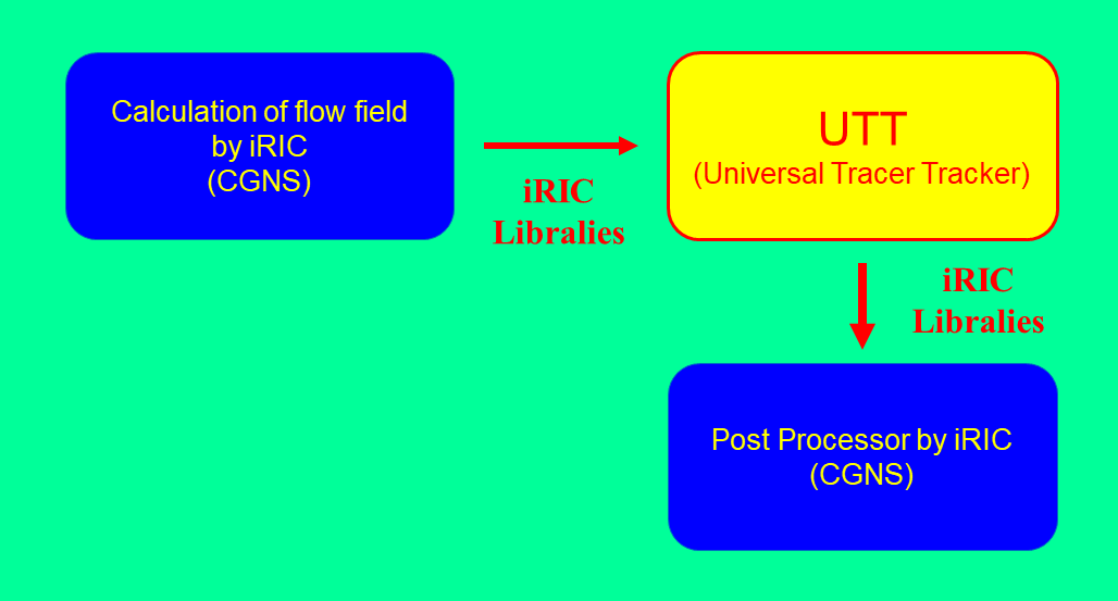
Figure 3 : Calculation Procedure by GELATO
The CGNS file that contains the calculation results of the flow used in GELATO is Specify from [Calculation conditions], [Settings], and [CGNS file to load flow calculation results] of the bar. (Figure 4)
Figure 4 : Specify the CGNS file which contains the calculation result of the flow
Computational grids used in GELATO
In most cases, the computational grid is imported from the CGNS files which contains the computational flow results. As shown in Figure 5 , from the “Object Browser” in the “Pre-Preprocessing Window”, Right-click [Grid(No data)], select [Import], and select a CGNS file which contains the grid information as Figure 6 . In most cases in iRIC, the file name is [Case1.cgn].
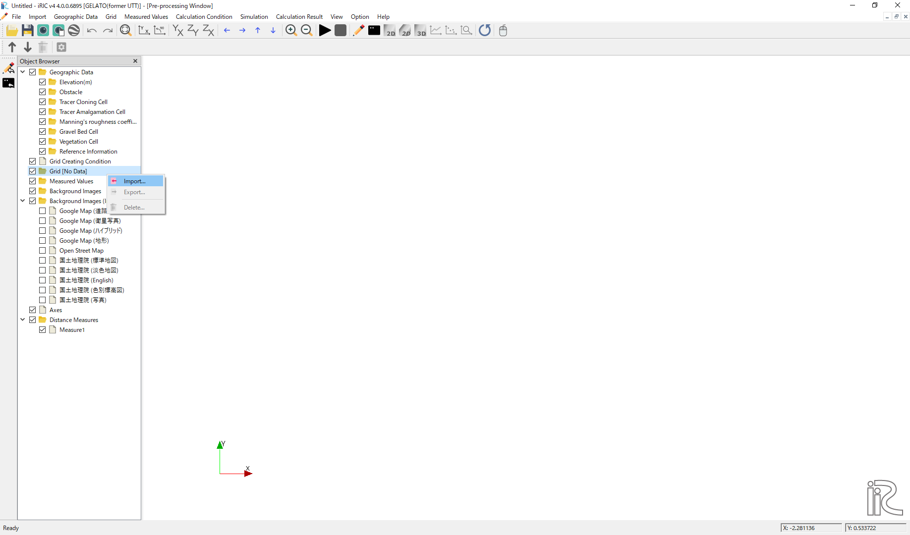
Figure 5 : Importing computational grid.
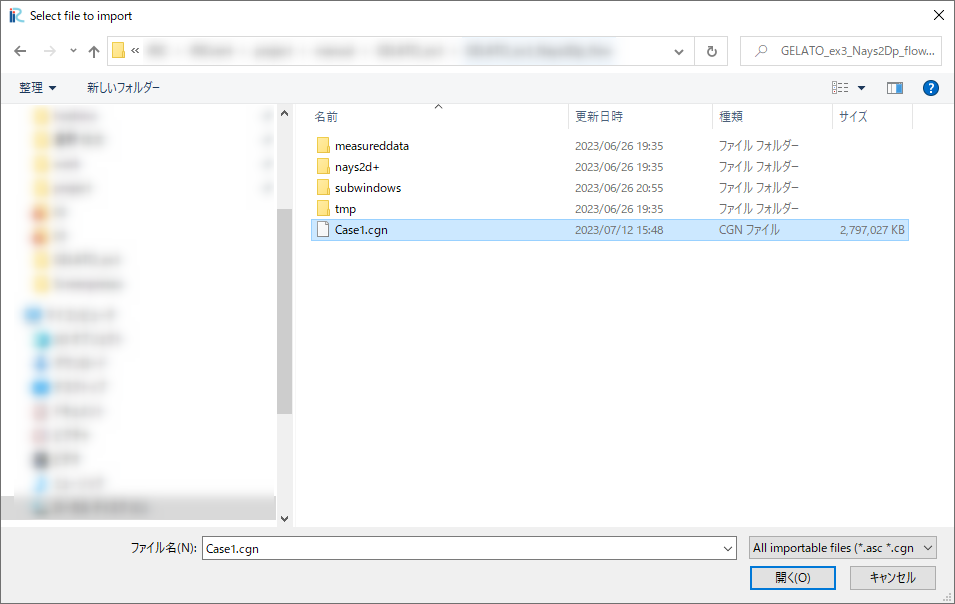
Figure 6 : Select a CGNS file
When you try to read the grid data from CGNS file produced by other than GELATO, Figure 7 is displayed. This means that the current project(GELATO project) is different from the flow calculation project. This is a warning that you are trying to import grids from a wrong project, but you can just click “OK”, and the grid information is imported and the result is displayed as Figure 8 .
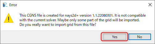
Figure 7 : Warning message
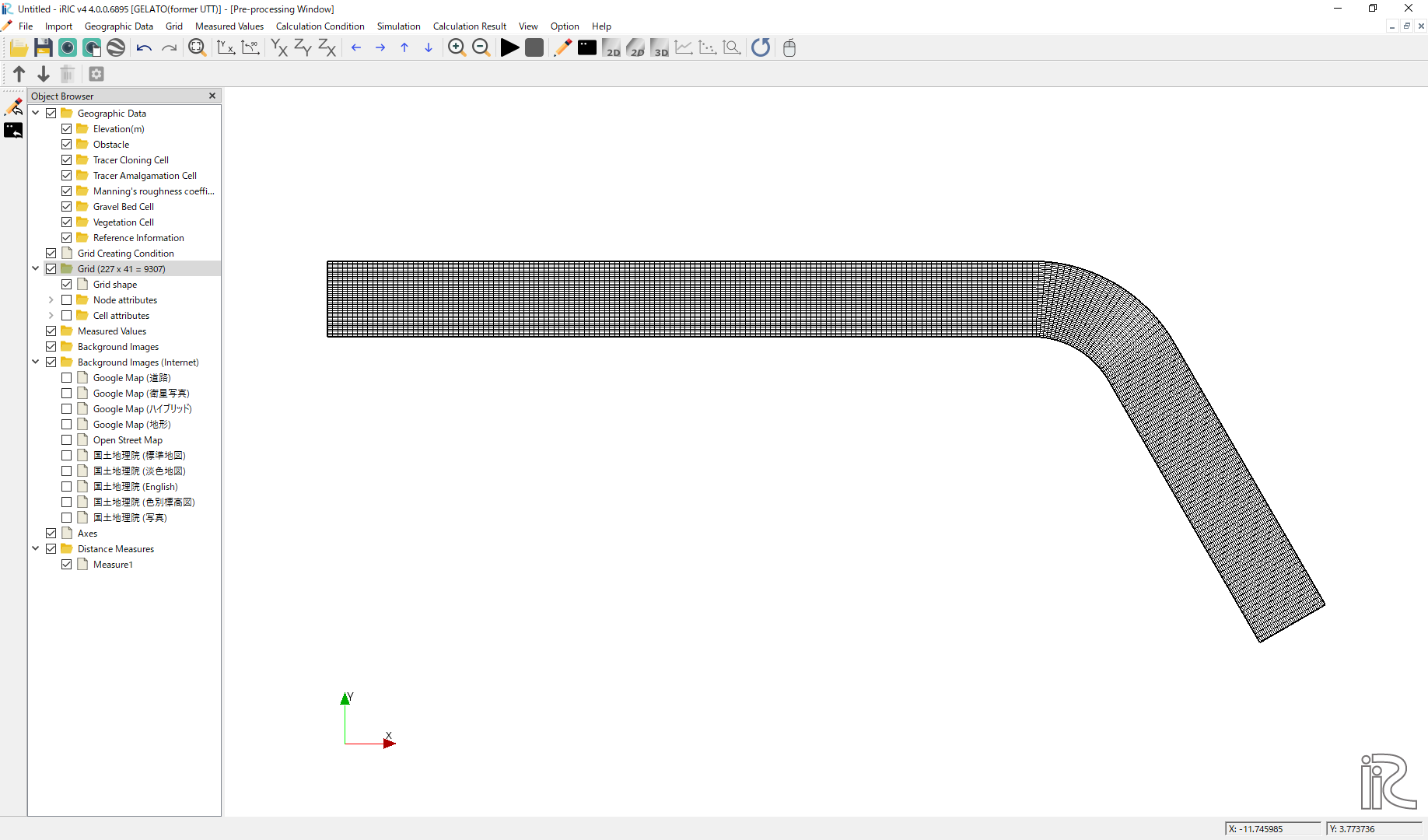
Figure 8 : Grid import completed
After this, the following procedure is used to calculate the tracer and display the result by GELATO. Examples are given in the next section.
Set computational condition
Calculation execution
Visualization of the solution