[Example 1] Tracer transport in a straight channel

Flow calculation by Nays2DH

Select a solver

In the [iRIC start page] , select [Create New Project], and when the [Select Solver] screen appears, choose [Nays2DH iRIC 4.x 1.0 64bit] and click [OK] button.

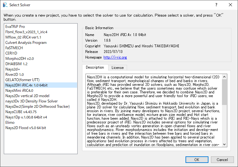
Figure 9 : Select Solver

A windows with “Untitled - iRIC 4.x.x.xxxx [Nays2DH]” appears as Figure 10.

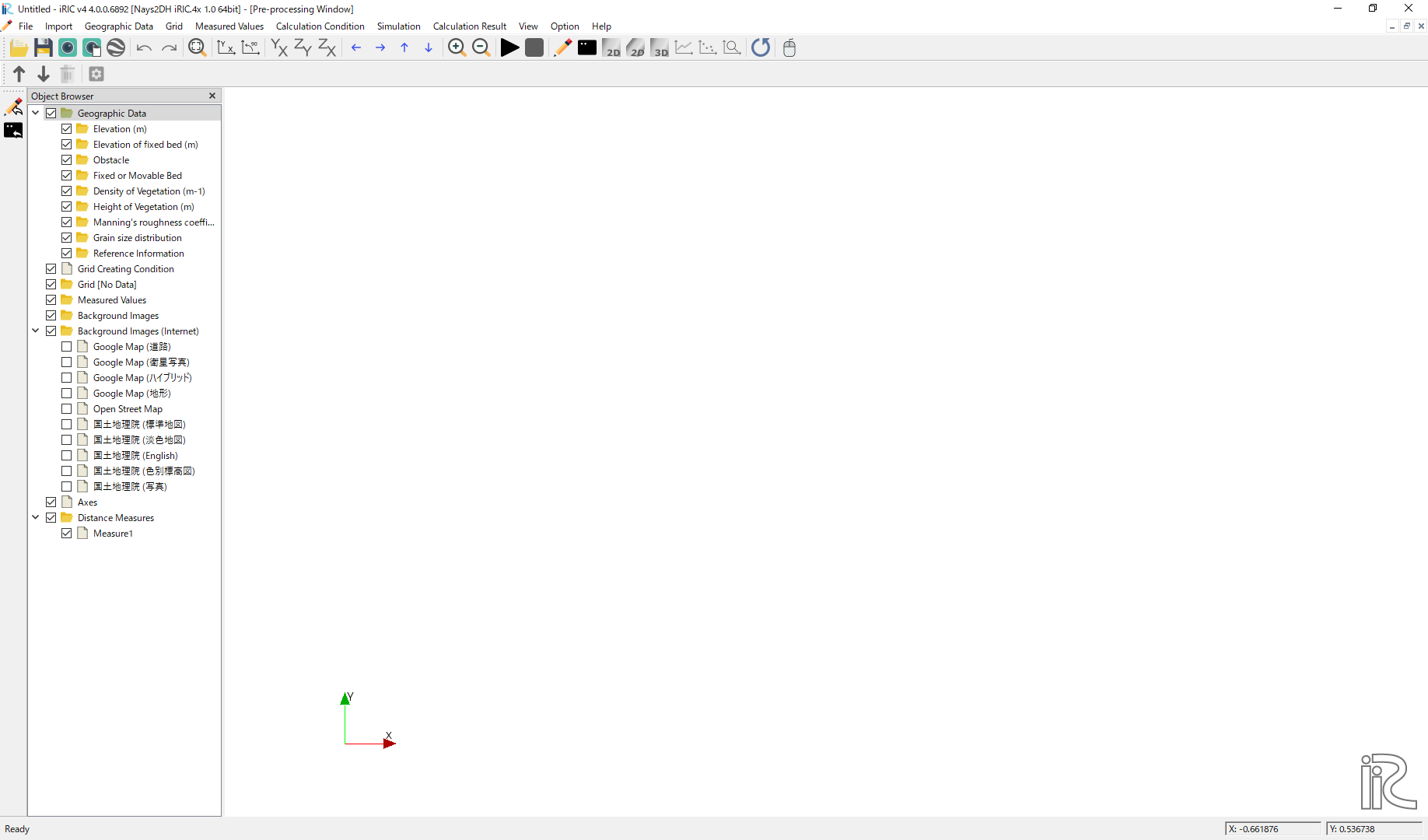
Figure 10 : Untitled

Grid Generation

From the main menu of the screen, Figure 10, choose [Grid]->[Select Algorithm to Create Grid] as Figure 11.

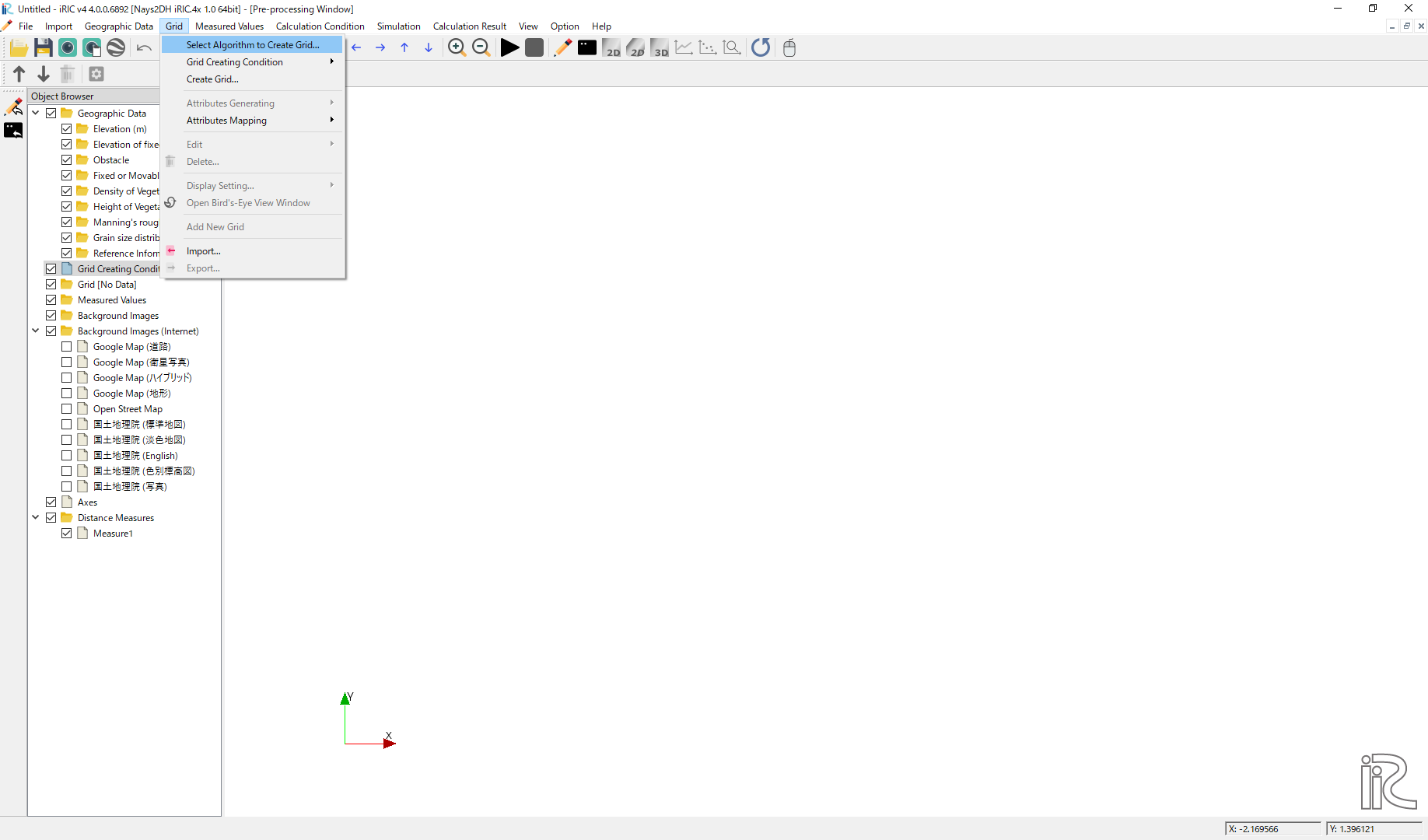
Figure 11 : Select Algorithm to Create Grid

In the [Select Grid Creating Algorithm] window, select [Simple Straight and Meandering Channel Creator] and click [OK] (Figure 12).

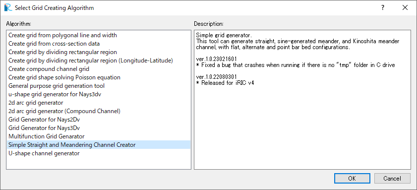
Figure 12 : Select Grid Creating Algorithm

In the window of Figure 13 , click “Channel Shape” and set [Select Channel Shape of the Main Part] as [straight channel], and other values as shown in Figure 13, then click [Create Grid].

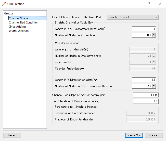
Figure 13 :Setting Channel Shape

When the confirmation window appears as Figure 14, click [Yes] to generate the grid, then the computational grid is generated as Figure 15 .

Figure 14 :Confirmation of mapping

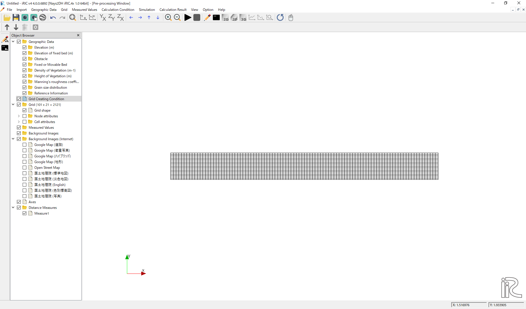
Figure 15 :Grid Generation Compete

Setting of calculation conditions for flow by Nays2DH

The next step is to set the calculation conditions. From the menu bar, select [Calculation Conditions]->[Settings], then the [Calculation condition setting window] as Figure 16 appears.

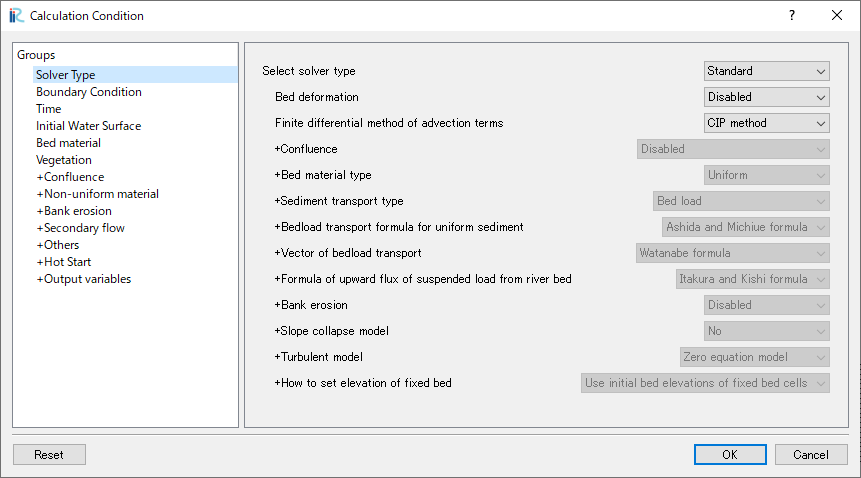
Figure 16 :Calculation Condition Window

As Figure 17, in the [Group] of the [Boundary Condition], click [Edit] at the [Time series of discharge at upstream and water level at downstream]. Then the [Time series of discharge at upstream and water level at downstream] appears as Figure 18 .

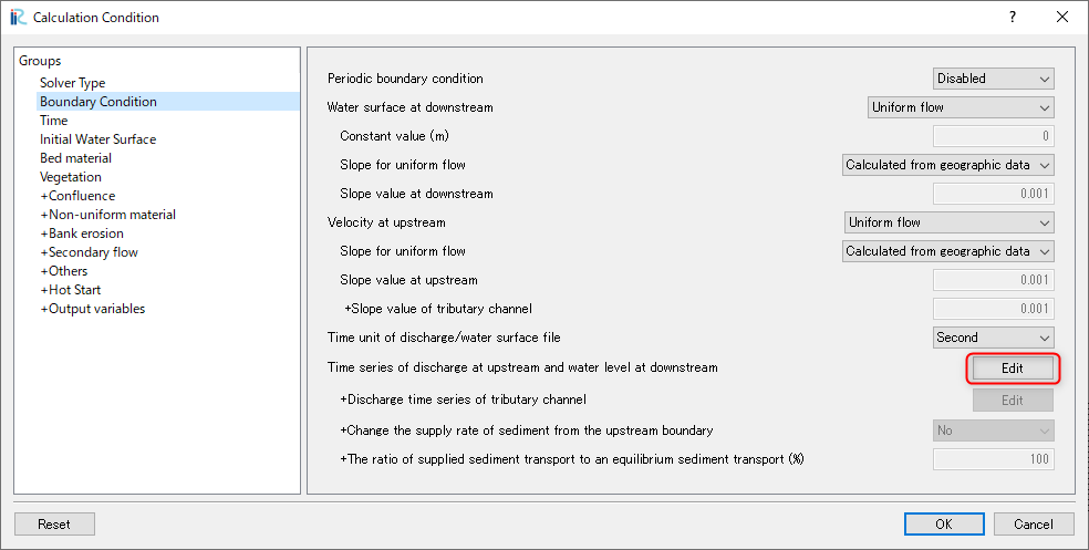
Figure 17 : Boundary Condition

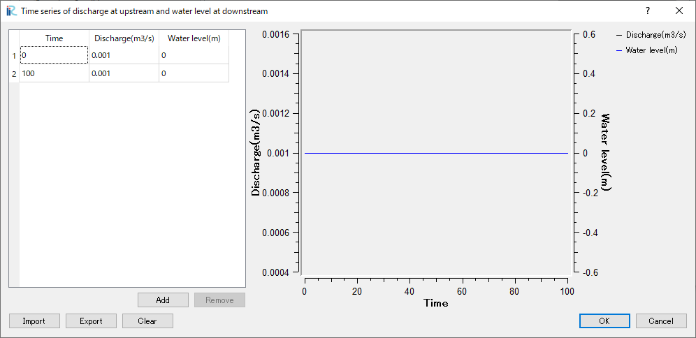
Figure 18 : Time series of discharge at upstream settings

In Figure 18, input [Time] and [Discharge] values, and click [OK] when you finish, and close this window.

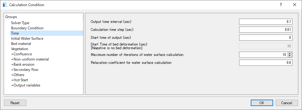
Figure 19 :Time parameters

Select [Time] and set parameters as Figure 19 and click [OK].

Flow calculation run by Nays2DH

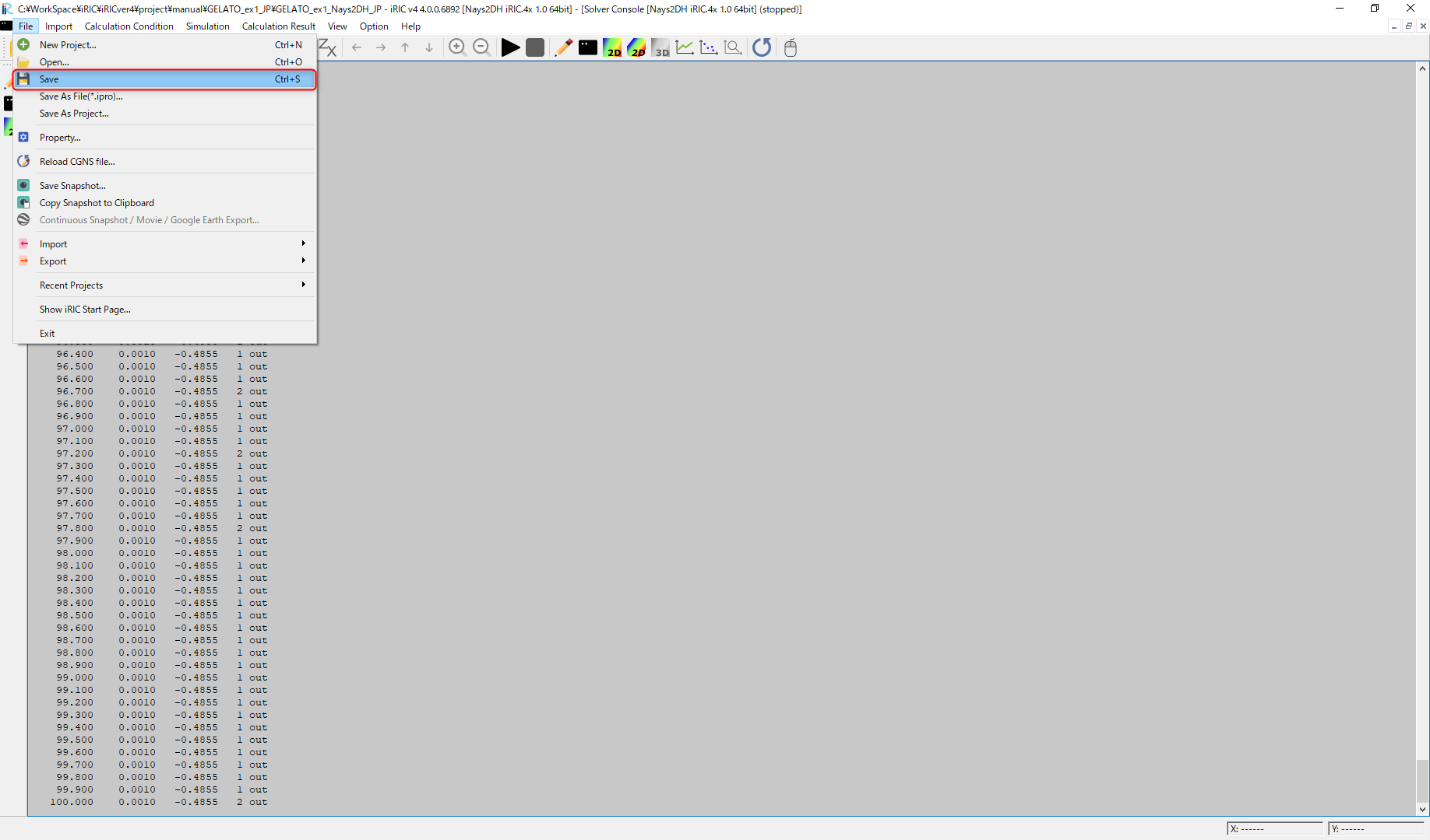
From the main menu, when you select [Simulation]->[Run], you will get the message like Figure 20 . Then, select [OK] and save the project with an appropriate name. At this time, do not save the project as an ipro file, but save it as a project.

Figure 20 :warning

A window as Figure 21 is shown during the computation, and Figure 22 appears when the computation is finished.

Then press [OK], and the computation is completed.

Figure 21 :Window when the solver is running

Figure 22 :Computation completed

Note

Whenever you finished the computation, select [File]->[Save] from the menu bar to save the results as Figure 23 . This result is important for later analysis by GELATO.

Figure 23 :Saving computational results

Visualization of the calculated results

After the calculation, select [Calculation Result] -> [Open New 2D Post-processing Window] to open the visualization window.

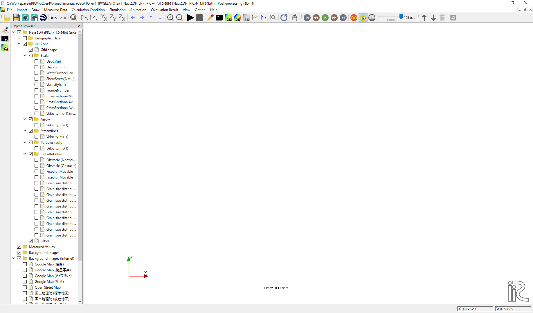
Figure 24 : 2D Post-processing Window

Velocity Vectors

In the [Object Browser], put check marks in the boxes by [Arrow] and [Velocity], click Focus on [Arrow] and click the right mouse button [Properties]. Vector setting” window as Figure 25 appears. Set the values in the red line and click [OK]. Figure 26 is the depth-averaged velocity vector. Here, the velocity distribution is uniform under the constant flow condition.

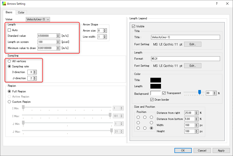
Figure 25 : Vector Settings

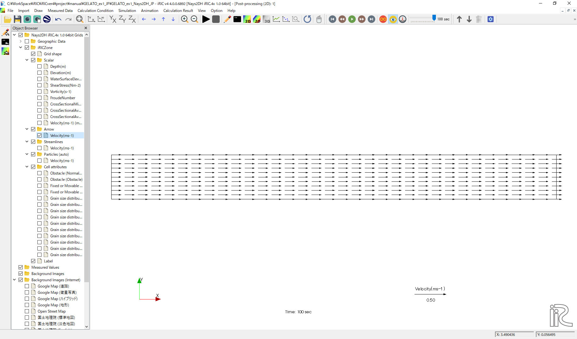
Figure 26 : Depth averaged velocity vectors

Display Particle Movement

Uncheck “Vectors” in the Object Browser, and put check marks in “Particles” and “Velocity” ( Figure 27 )

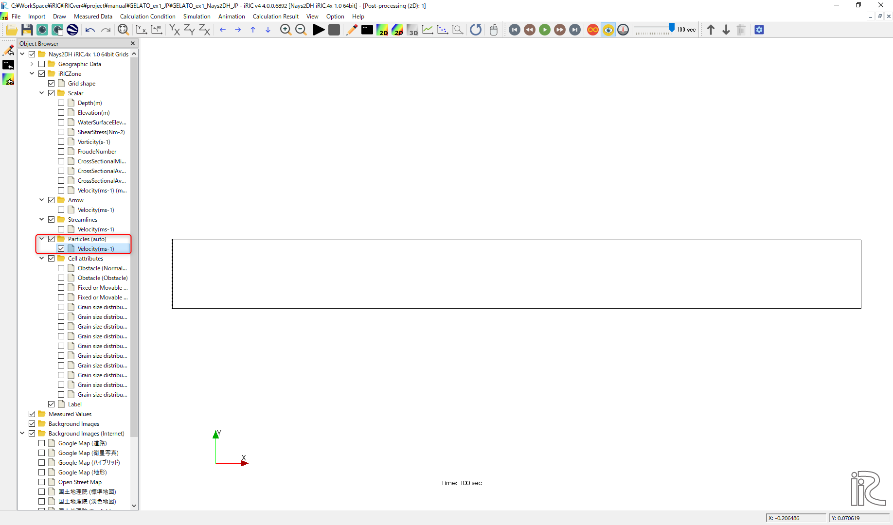
Figure 27 : Particles(1)

Right click [Particle] and select [Properties] as Figure 28 .

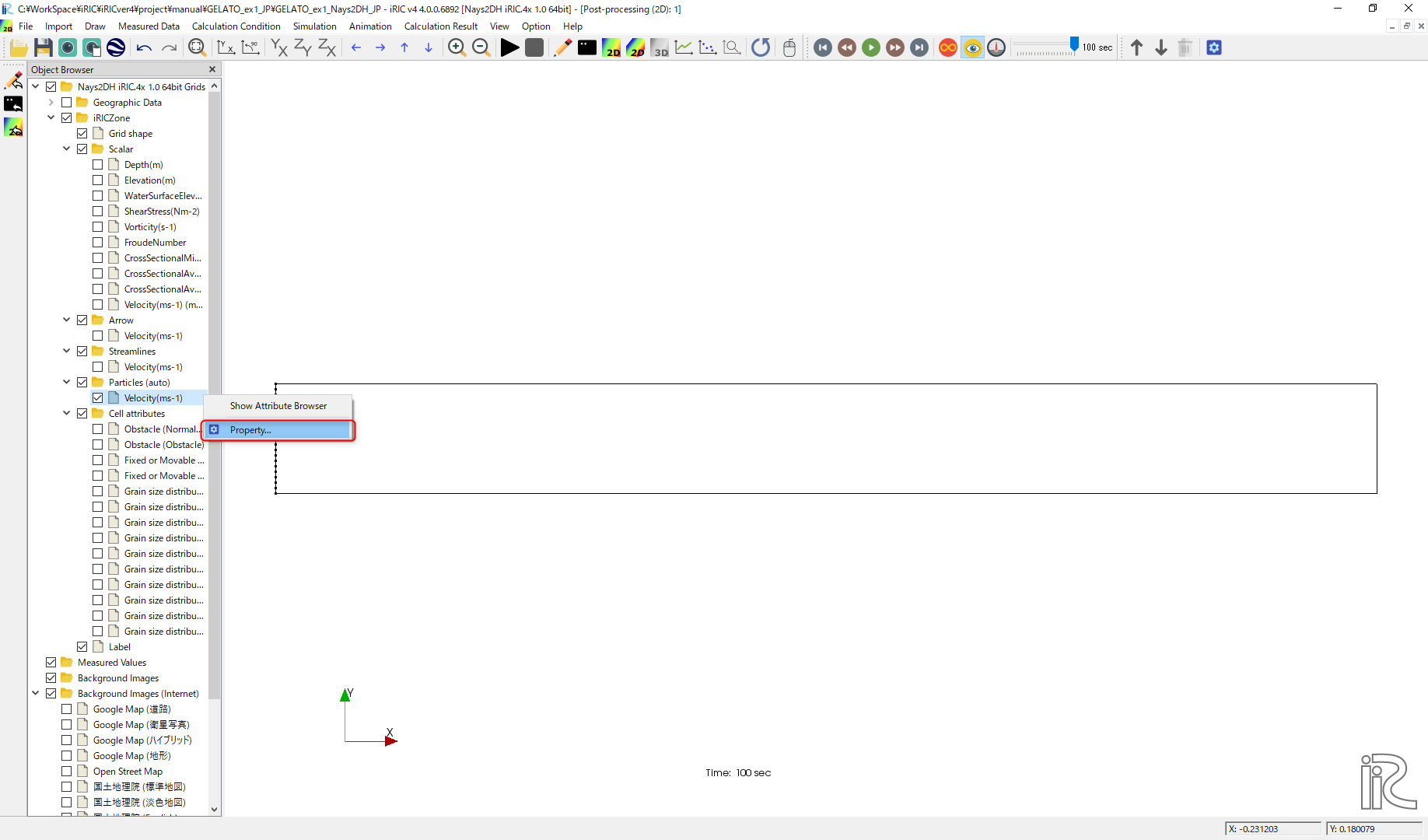
Figure 28 : Particles(2)

Set parameters for particle injection as shown in red box in Figure 29 .

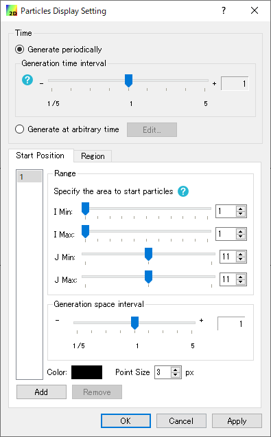
Figure 29 : Set particle parameters

As shown in Figure 30 , set time bar back to zero, and select [Animation]->[Start/Stop Animation] rom the main menu bar. Then the particle animation starts.

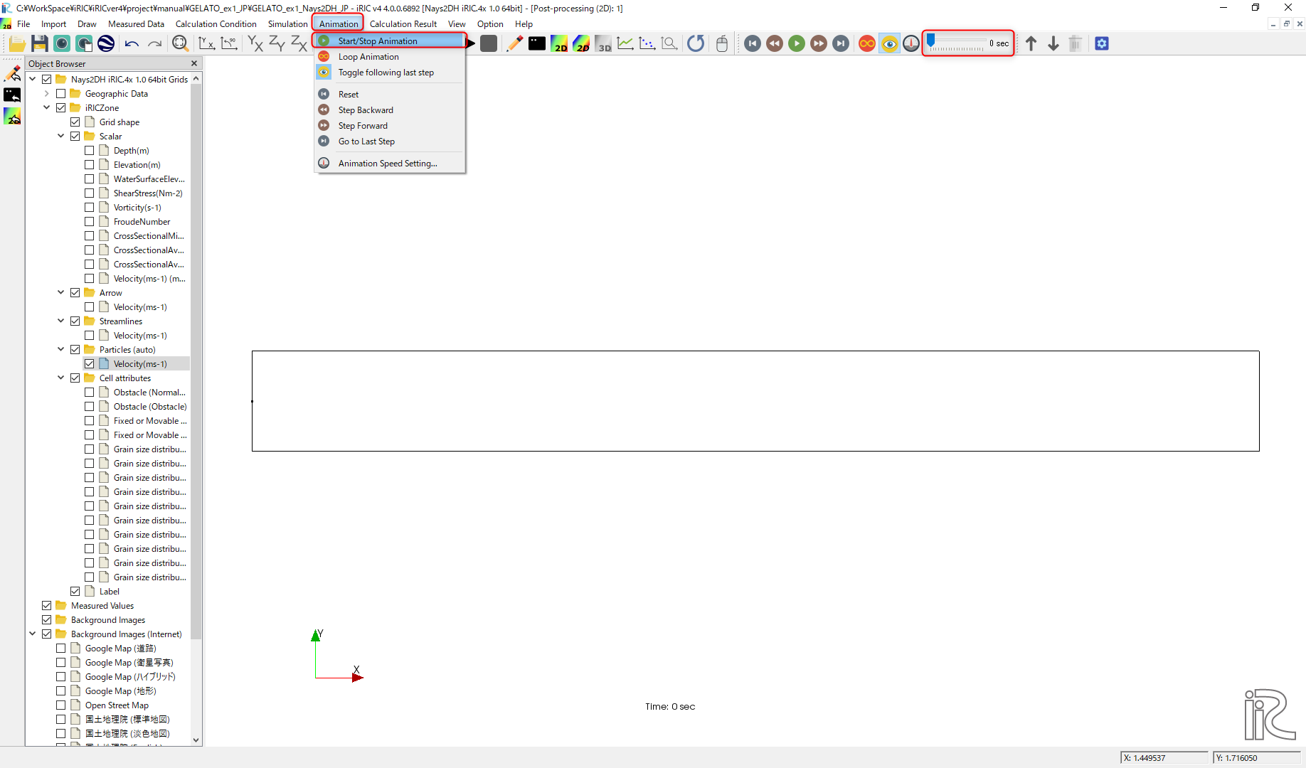
Figure 30 : Start Particle Animation

Figure 31 : Particle animation by Nays2DH

As can be seen in Figure 31, since the sub-grid scale turbulence is not included in the output velocity from the solver. It only shows very simple steady and uniform movement.

Tracer Tracking by GELATO

Starting GELATO

From the iRIC startup screen, select [New Project], and in the solver selection screen appears. Select “GELATO” and click “OK” ( Figure 32 ).

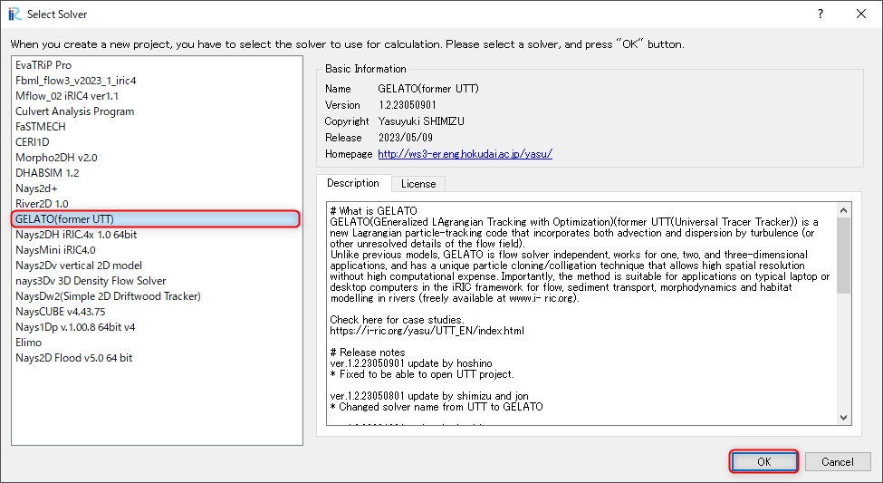
Figure 32 : Selecting GELATO and Starting

A window with [Untitled -iRIC 4.x.xxxx] [GELATO] appears, and the GELATO session is started. (Figure 33 )

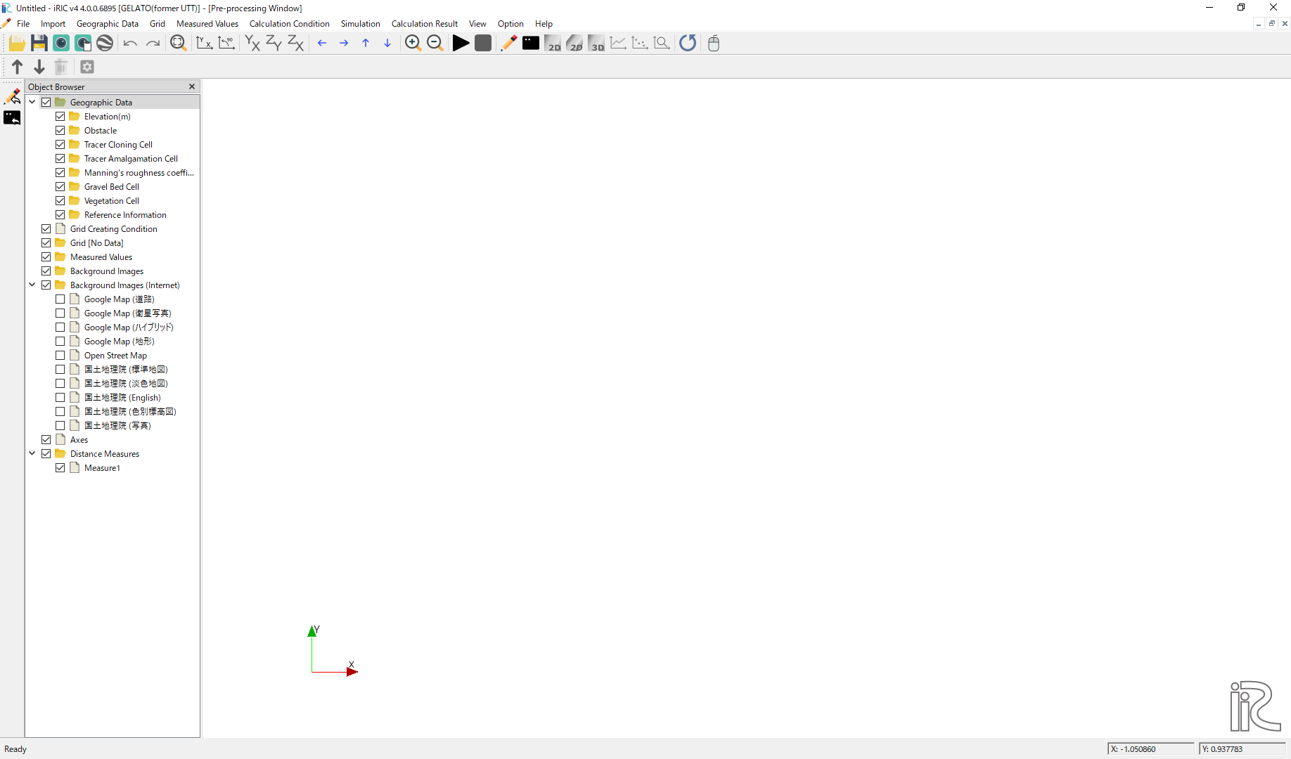
Figure 33 : Opening GELATO

At this stage, the [Grid] in the [Object Browser] shows [No data] as shown in Figure 33 , we will first import the grid data created in Grid Generation session.

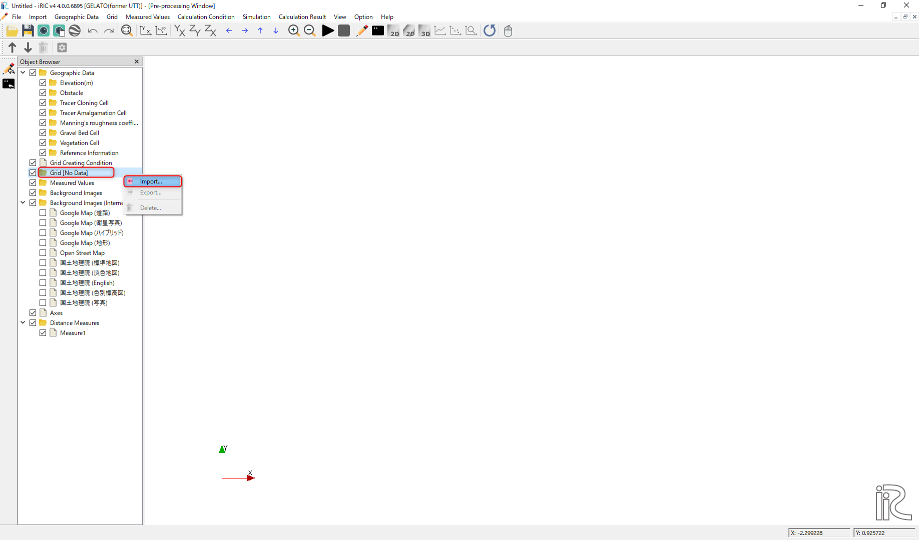
Figure 34 : Grid data import

Right click [Grid(No Data)] and select [Import] as (Figure 34 ).

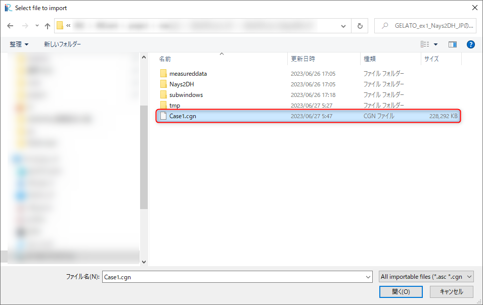
Figure 35 : Select CGNS file contains grid data

As shown in Figure 35, select [Case1.cgn] which contains the grid data used in the previous section of [Computational Results of Nays2DH], and click [Open].

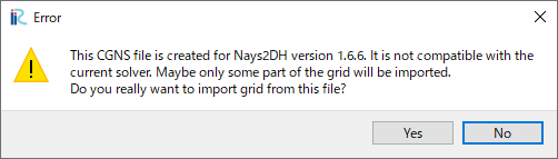
Figure 36 : Warning Message

A warning message is coming out as Figure 36 , Just click [Yes] without worry, and the grid import is completed as Figure 37 .

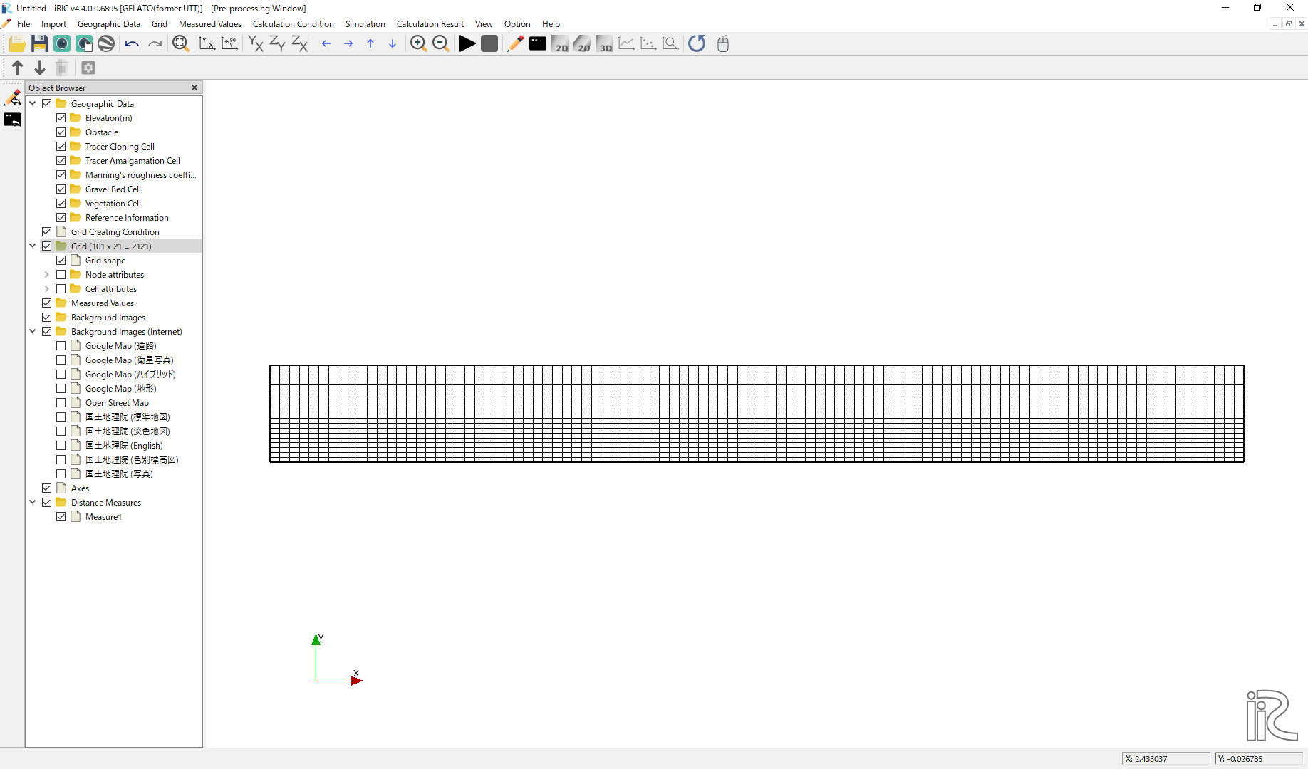
Figure 37 : Grid import completed

Single Tracer Tracking(Without Turbulent Diffusivity)

Condition Settings

Choose [Calculation Condition]->[Setting] as Figure 38

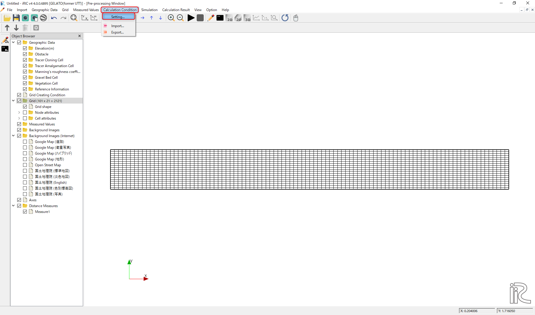
Figure 38 : Calculation Condition Settings(0)

Set parameters as follows.

[Flow information file name] is Locat of the CGNS file to read the calculation result of the flow field. Here, the CGNS file produced by the Nays2DH computation.( Flow calculation run by Nays2DH ).

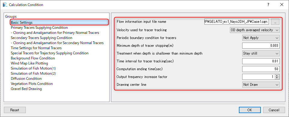
Figure 39 : Basic Settings

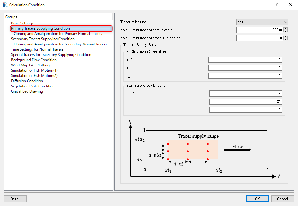
Figure 40 : Primary Tracers Supplying Condition

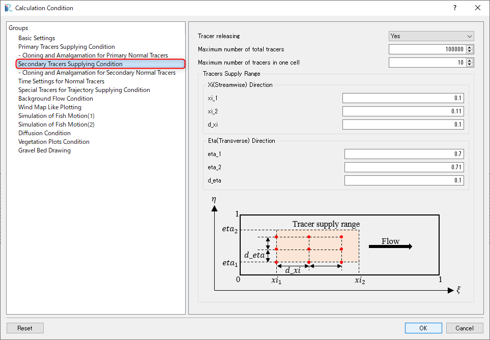
Figure 41 : Secondary Tracers Supplying Condition

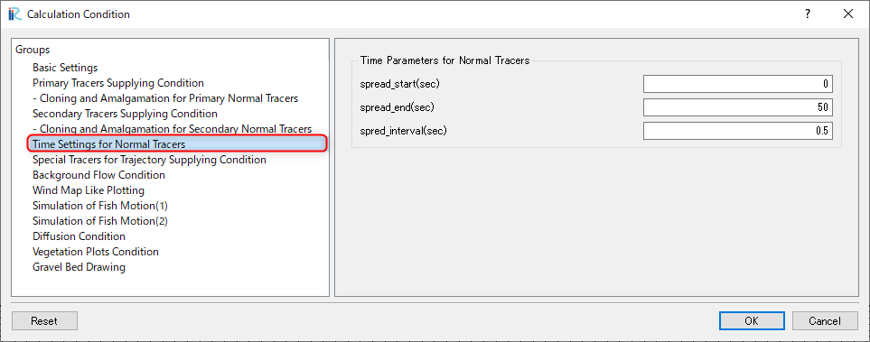
Figure 42 : Time Settings for Normal Tracers

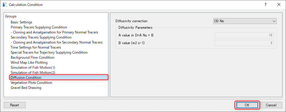
Figure 43 : Diffusion Condition

Launch GELATO

From the main menu bar, select [Simulation]->[Run], then you are asked as Figure 44. When you click [OK] and save project, the computation starts as Figure 45.

Figure 44 : warning

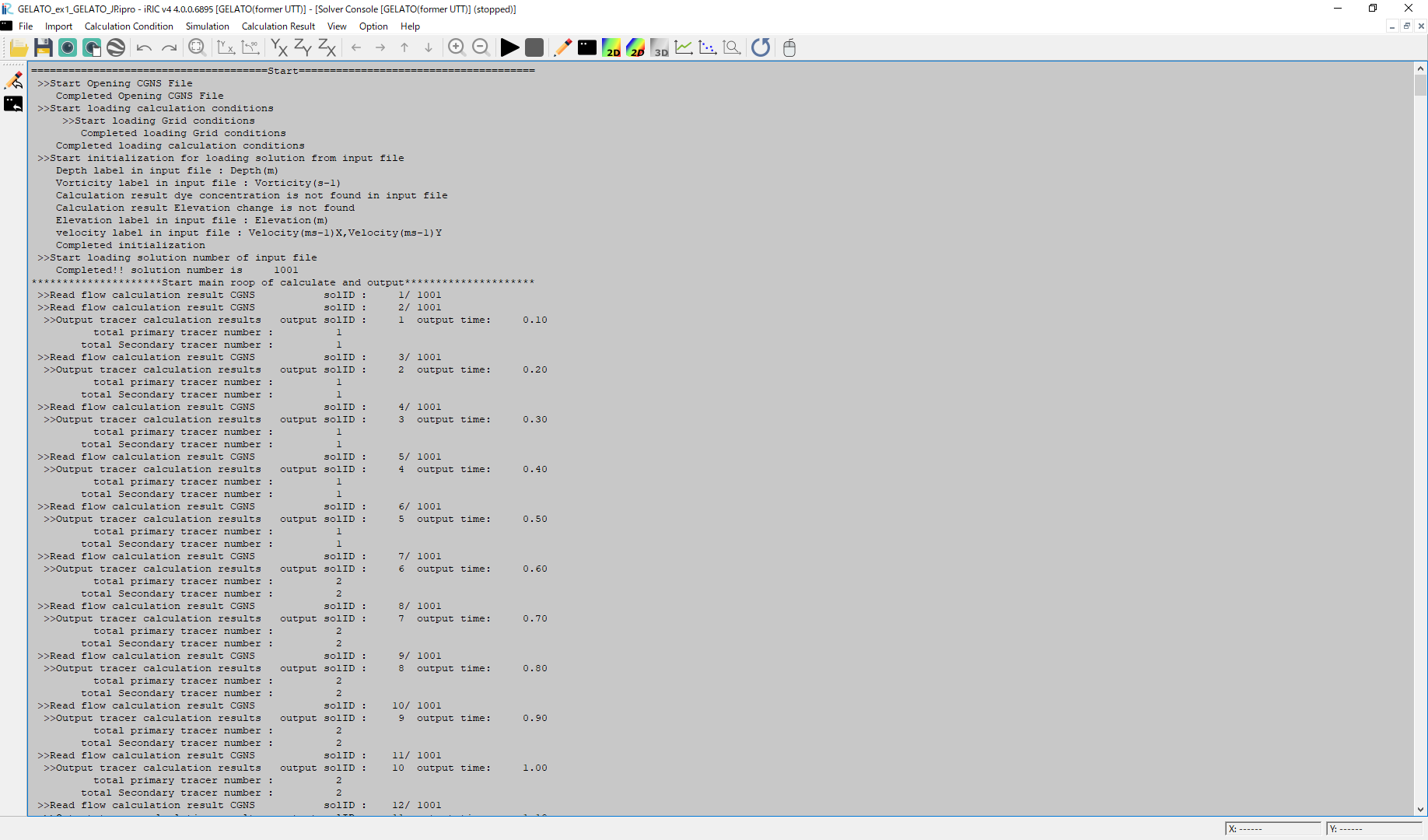
Figure 45 : Launch GELATO

When the computation finishes, Figure 46 appears, and click [OK] for confirmation.

Figure 46 : Computation finished

Visualization of Computational Results

From the main menu, select [Calculation Result]->[Open ne 2D Post-processing Window] as Figure 47, then [2D Post Processing Window] will appear.

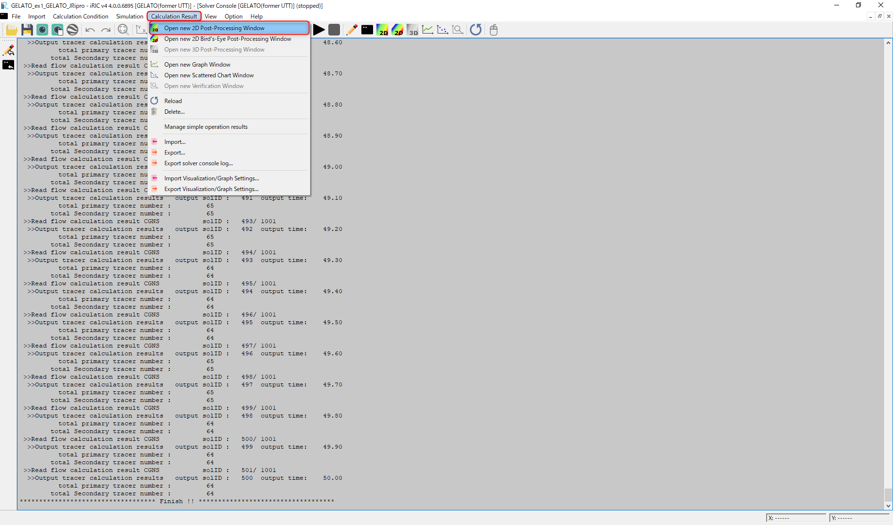
Figure 47 : Open 2D Post Processing Window

Right-click [Primary Nomal Tracers] and [Secondary Nomal Tracers] in the [Object Browser] and click [propertie].

Then [Particles Scalar Setting] that appears,and you can set the primary and secondary have different colors by setting like Figure 48.

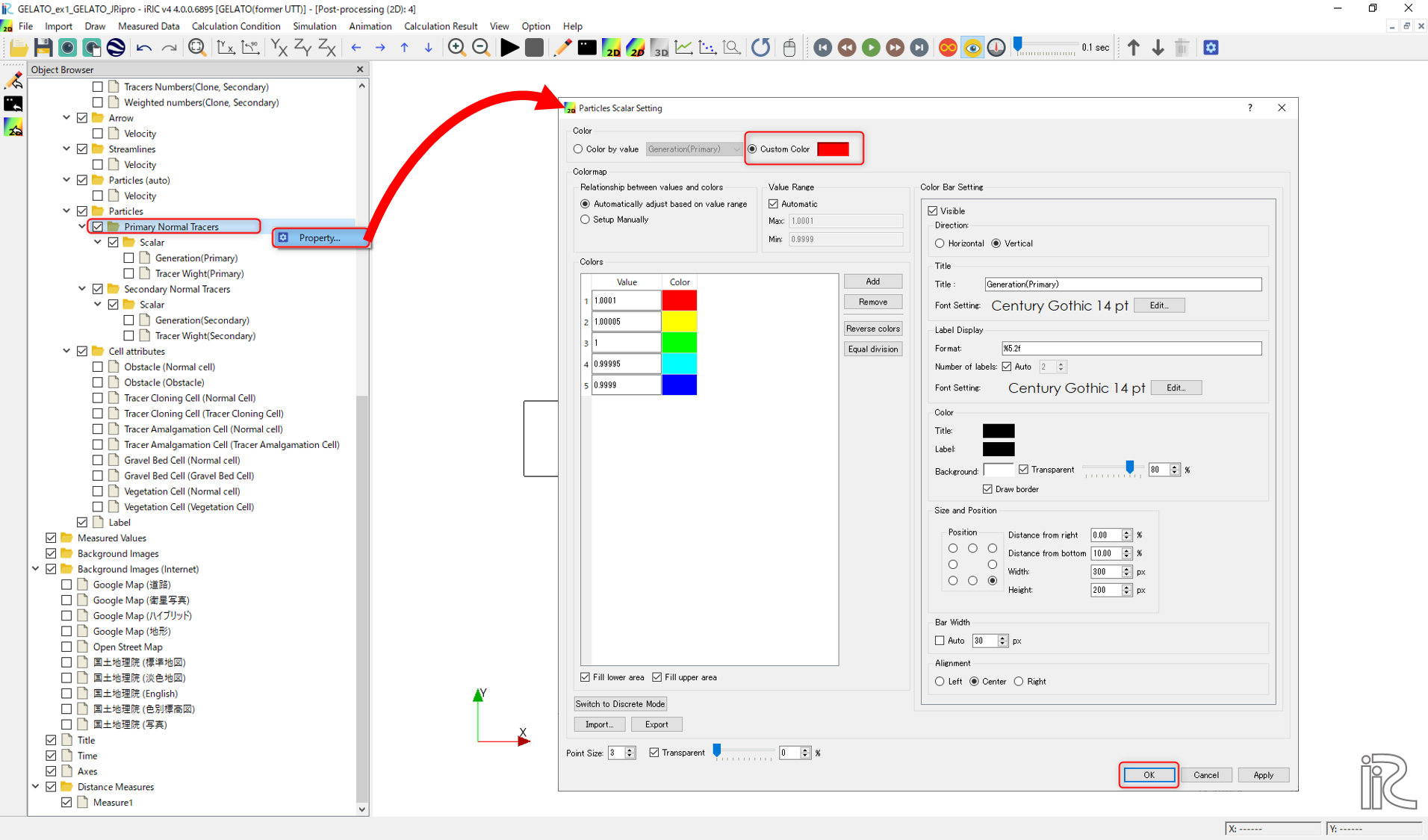
Figure 48 : Setting particles colors

From the main menu, select [Animation]->[Start/Stop] as Figure 49, animation starts ( Figure 50 ).

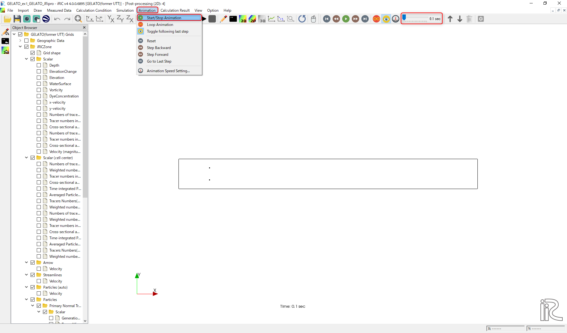
Figure 49 : Visualization of computational results

Figure 50 : Tracer movement(No diffusivity)

It is obviously very simple because it doesn’t including any turbulent effect (Figure 50).

Single Tracer Tracking(With Turbulent Diffusivity)

Setting Computational Condition

Change the calculation conditions to take into account for the effect of turbulent diffusion. From the main menu, select [Calculation Conditions] → [Setting], and show the Figure 51. check the box of [Diffusion Condition]->[Diffusivity Correction] , set the parameter [A Value] to [1], and then click “OK”.

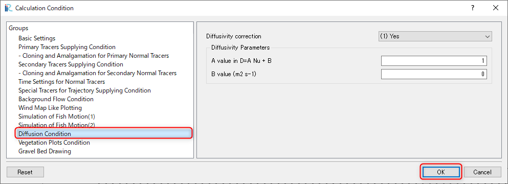
Figure 51 : Calculation Condition (Diffusion Condition)

Launch GELATO and the Results Visualization

Computation can be conducted through the same procedure as previous example, the animation becomes as Figure 52.

Figure 52 : Tracer Movement(With Turbulent Diffusivity A=1)

When the value of A is set as [10], the results become as Figure 53, the effect of the turbulent becomes stronger.

Figure 53 : Tracer Movement(With Turbulent Diffusivity A=10)