[Example 3] Tracer Tracking Simulation in Real River

In this section, we perform s simulation of tracking floats for the discharge measurements in a real river. Floats are injected from a bridge and velocities are calculated by measuring the flow time between two sections ste up with 100m interval in which the upper section is located 130m downstream of the bridge. Using a discharge of 384m \(^3\)/s, flow calculation is conducted using Nays2d+, and the paths of the floats are simulated by GELATO.

Flow Calculation by Nays2d+

Selection of Solver

From the start window of the iRIC, launch [Nays2d+] as Figure 169.

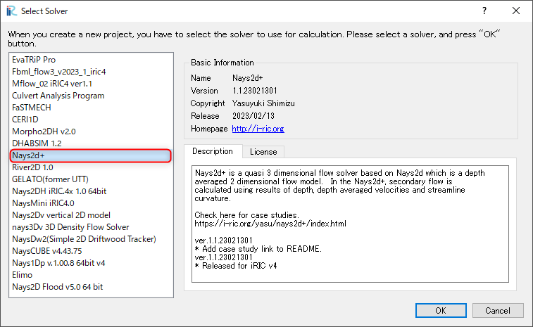
Figure 169 : Solver Selection

Import Geometric Data and Making Computational Grid

Importing River Bed Elevation Data

From the main menu, select [Import]->[Geographic Data]->[Bed Elevation(m)] as Figure 170, and read “tikei.tpo (Point Claud Data)” as shown in Figure 171.

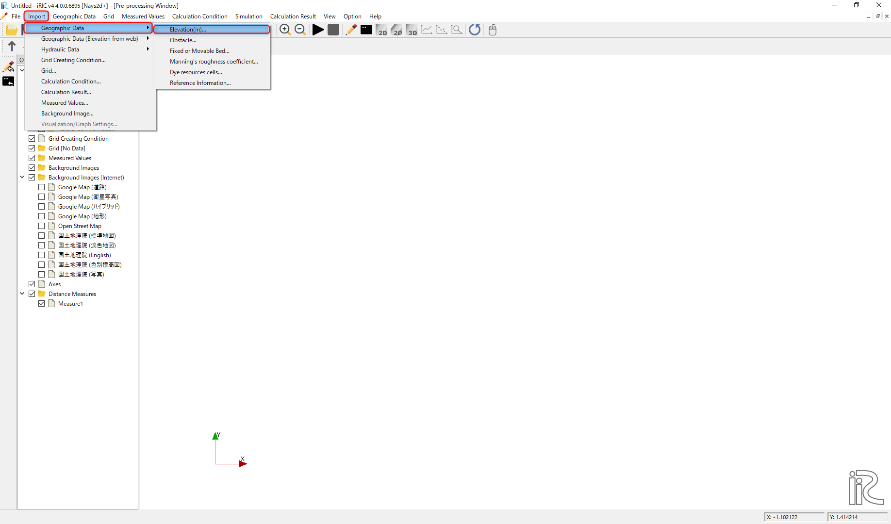
Figure 170 : Import River Bed Data File

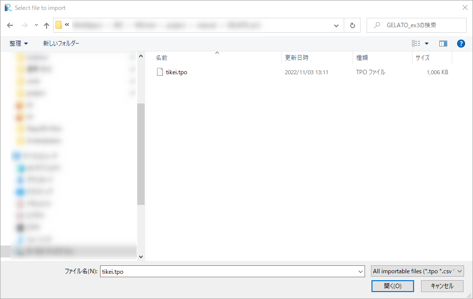
Figure 171 : Selecting a tpo file

While reading the data, you need to set filtering value as Figure 172. In this example, choose [1] just for without filtering.

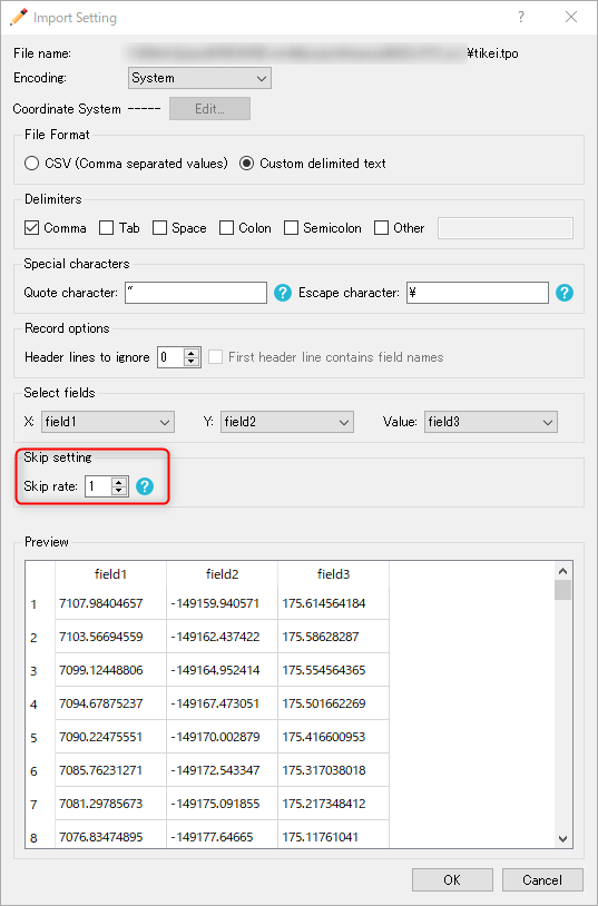
Figure 172 : Input Filtering Value

The geometric data (ground elevation data) is shown as Figure 173.

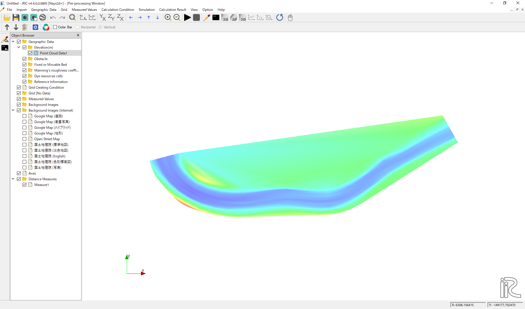
Figure 173 : Geometric Data

Setup Background image

From the main menu, select [File]->[Property], and press [Edit] button at [Coordinate System:] information as Figure 174.

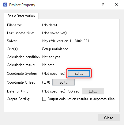
Figure 174 : Project Property

in the [Select Coordinate System] window, type “Japan” at [Search:] box, and select [EPSG ….. Japan …. IV] from the list below the [Search:] box, and press [OK] as Figure 175. Then close the [Project Property] window by pressing [Close].

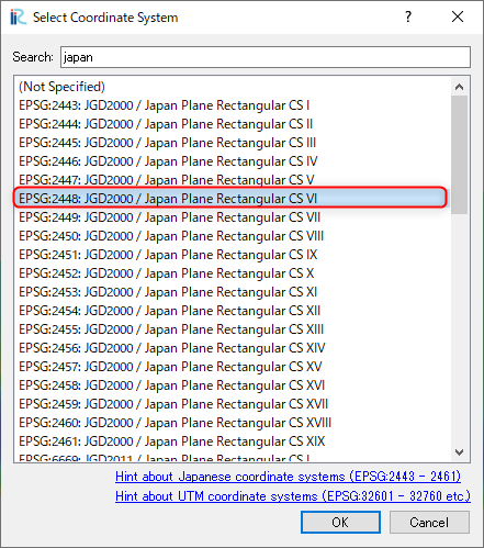
Figure 175 : Select Coordinate System

In the [Object Browser], put check marks at [Background Images (Internet)] ->[国土地理院(標準地図)] as Figure 176.

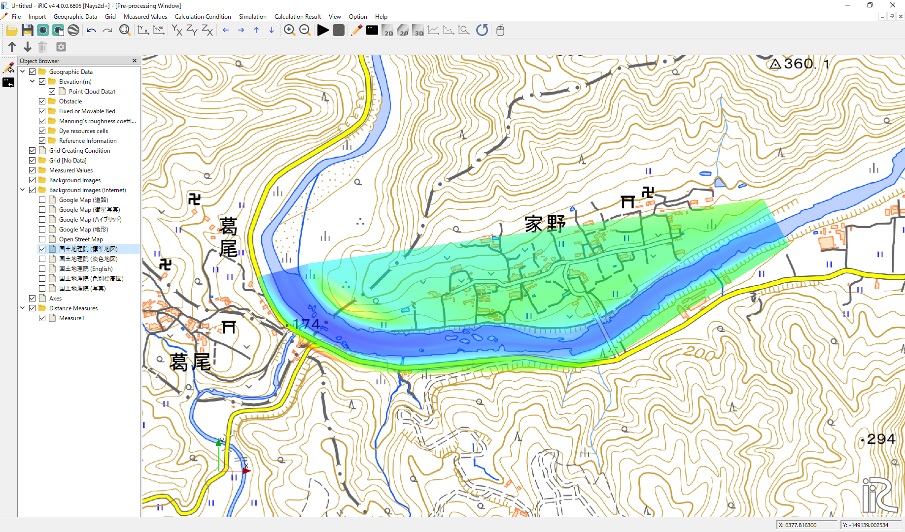
Figure 176 :Select Background Image

Grid Creation

From the main menu, select [Grid]->[Select Algorithm to Create Grid], and select [Create grid from polygonal line and width] in the next window (Figure 177)

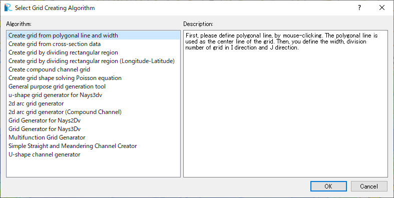
Figure 177 : Select Grid Creating Algorithm

Assign channel center points from the upstream side to down stream side as Figure 178.

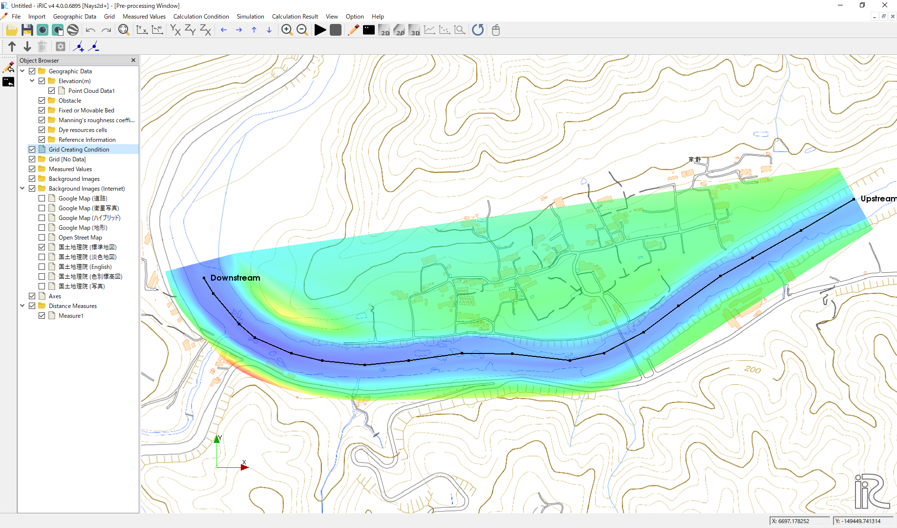
Figure 178 : Assign Center Points

In the [Grid Creation] window, Figure 179, input values as Ni=290, Nj=56 and W=140, then the grid size becomes about 2.5mx5.0 m as Figure 180.

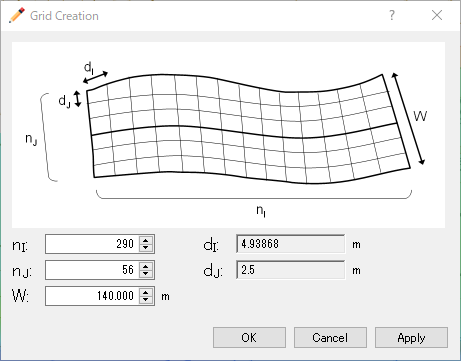
Figure 179 : Grid Creation

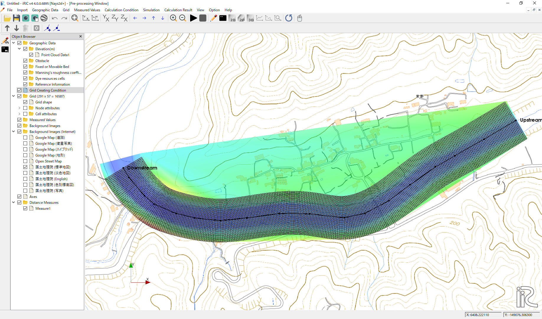
Figure 180 : Created Grid Shape

Setup for Bridge Piers

From the [Object Browser] in the left side of the window, hide the [Point Cloud Data 1] by removing the check mark. Right click [Obstacles], select [Add]->[Polygons], and make polygons by clicking the outer edge of the piers, and assign them as [Obstacle] (Figure 181) Surround all the cells in one polygon and assign it as [Normal Cell]. Note that the [Normal Cell] polygon has to be located at lower layer than the [Obstacle] polygons (Figure 182).

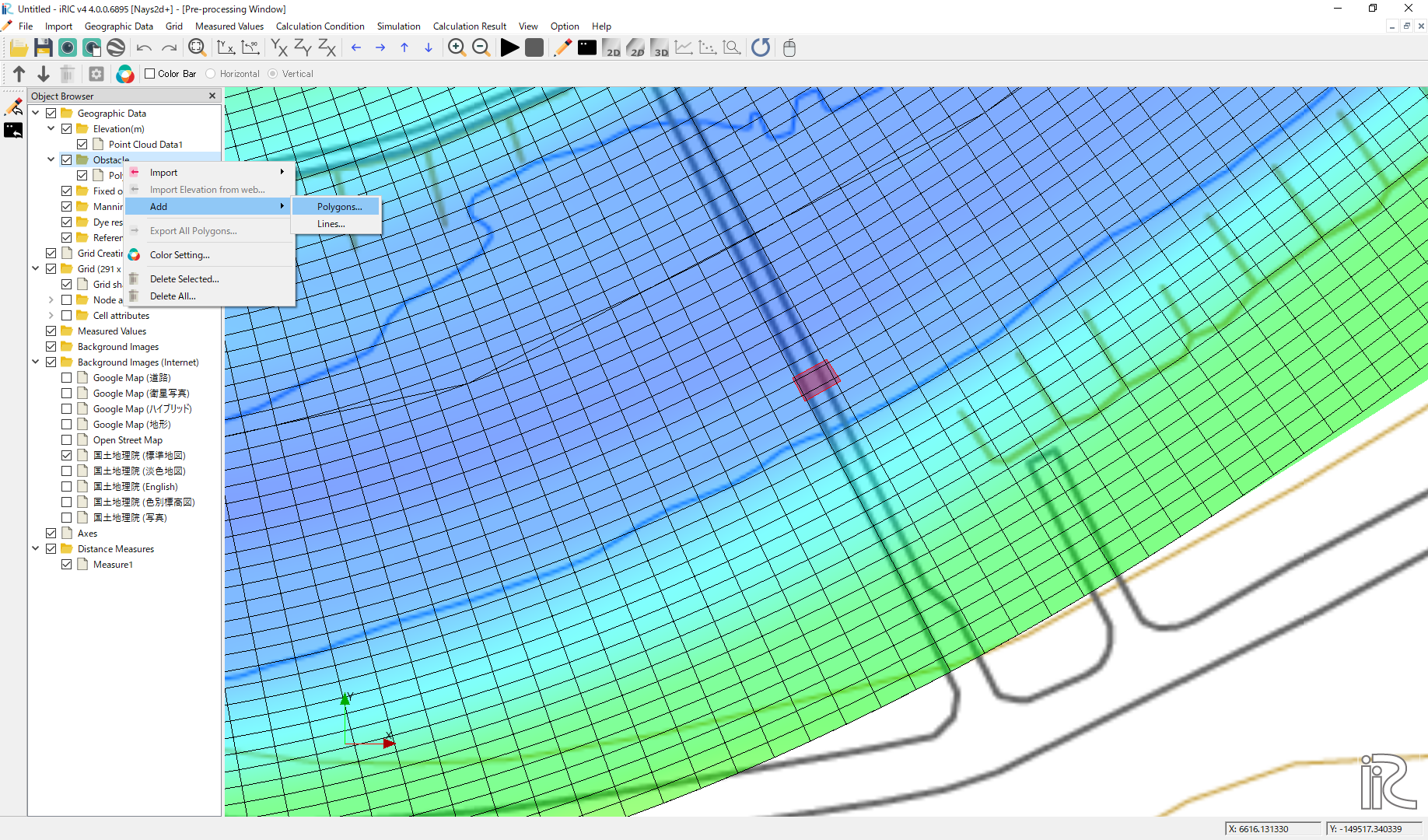
Figure 181 :Obstacle Cells for Bridge Piers

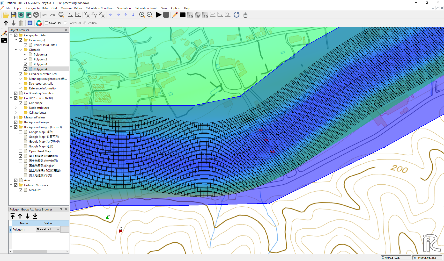
Figure 182 :Normal Cells for All the Area

Set Manning’s Roughness Coefficient

In the [Object Browser] under the group of [Geographic Data], right click [Manning’s roughness coefficient] and select [Add]->[Polygons], and make a polygon covering all the grid domain, and input n=0.030 (Figure 183).

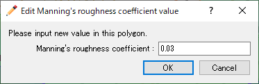
Figure 183 :Set Manning’s Roughness Coefficient

Attributes Mapping

From the main menu, select [Grid]->[Attributes Mapping]->[Execute] (Figure 184).

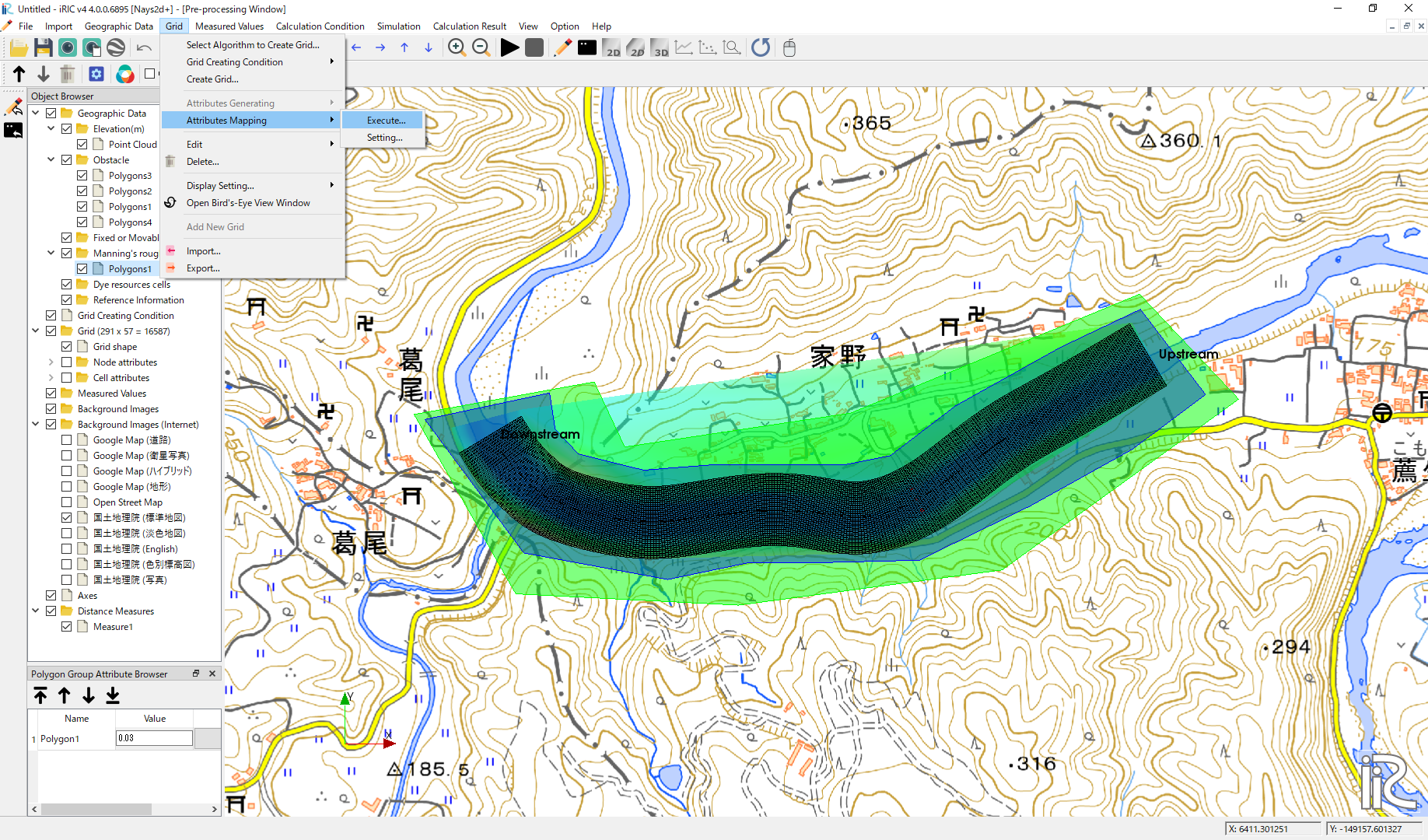
Figure 184 :Select Attributes Mapping

Put check marks at [Elevation(m)], [Obstacle] and [Maninng’s roughness coefficient] in the [Attribute Mapping] window as Figure 185, and press [OK] to execute mapping.

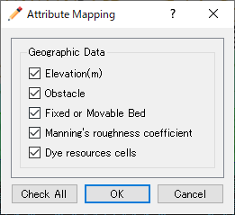
Figure 185 :Choose Mapping Items and Execute Mapping

Set Calculation Condition

From the main menu, select [calculation Condition]->[Setting], and input parameters in the [Calculation Condition] window as the following figures of Figure 186, Figure 187, Figure 188, Figure 189, Figure 190 and Figure 191. When you finished to input parameters, press [OK].

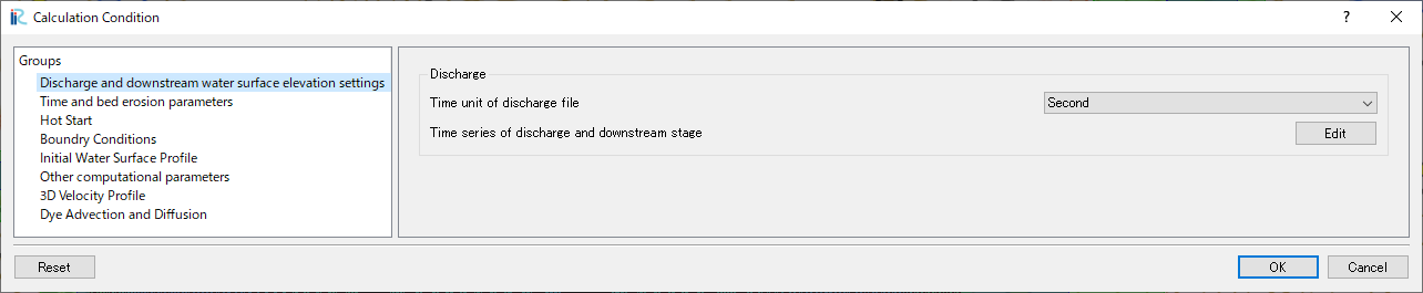
Figure 186 :Discharge and downstream water surface elevation settings

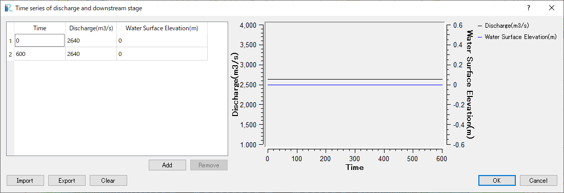
Figure 187 :Time series of discharge and downstream stage

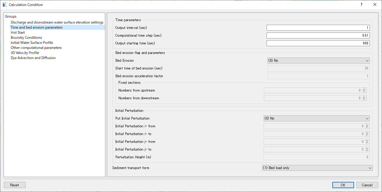
Figure 188 :Time and bed erosion parameters

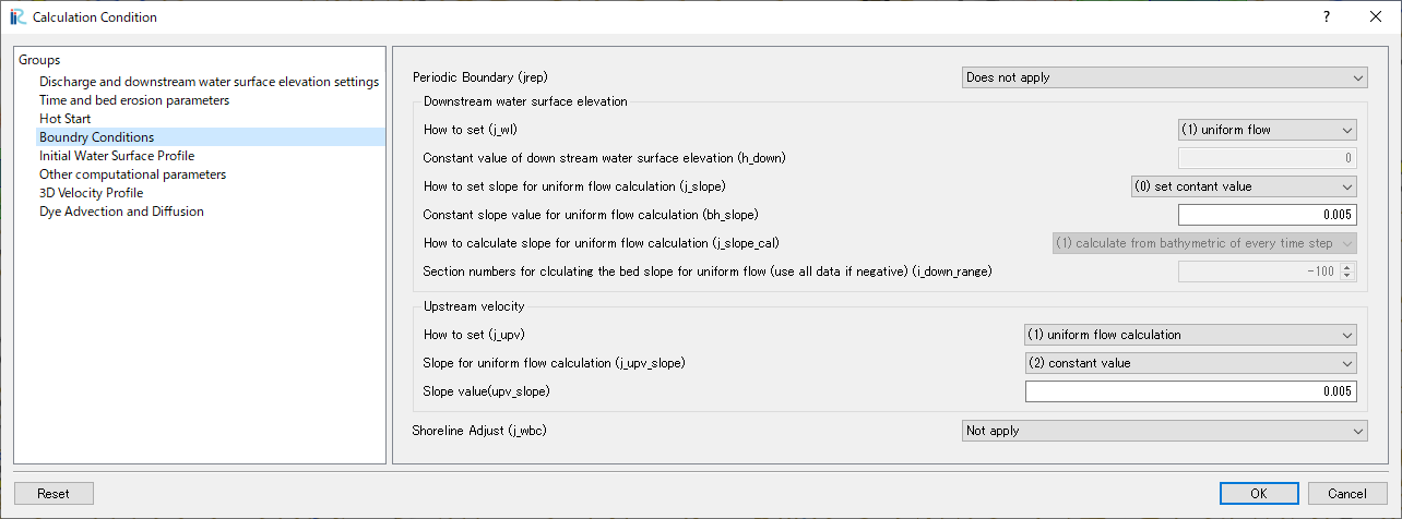
Figure 189 :Boundary Condition

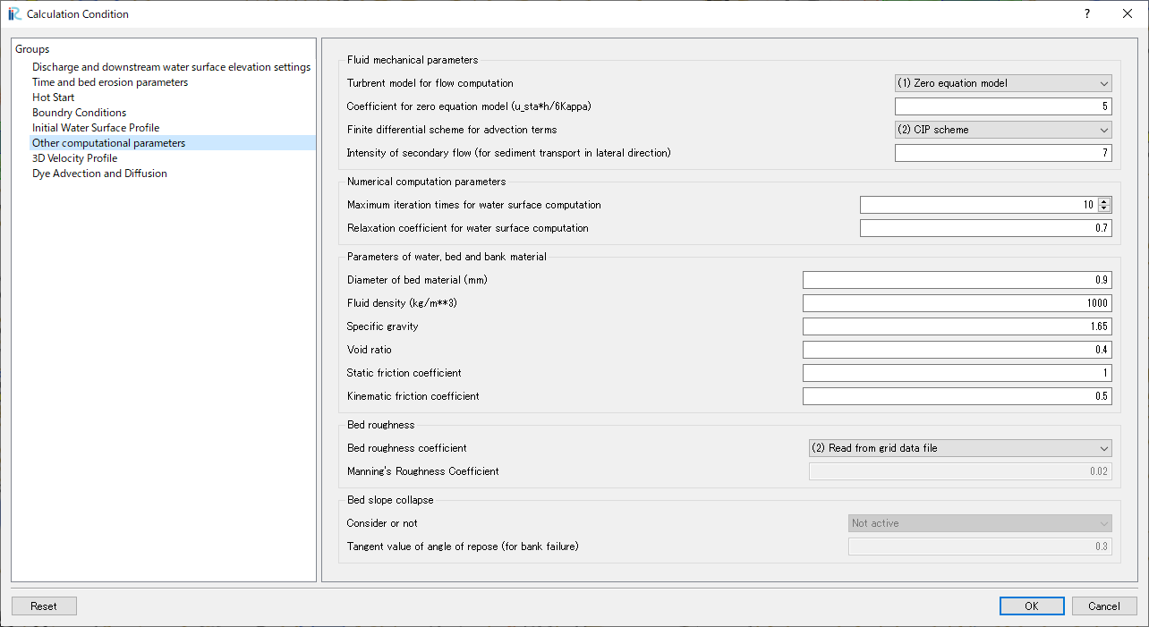
Figure 190 :Other computational condition

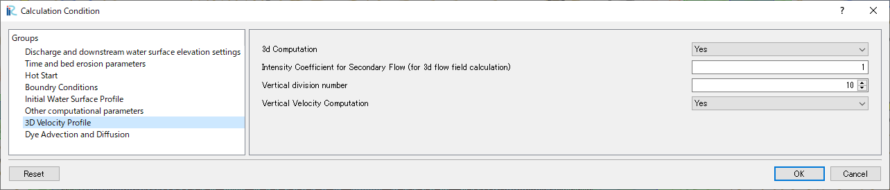
Figure 191 :3D Velocity Profile

Execute a Solver

Save the project with some name, and run the solver by [Simulation]->[Run]. When the simulation finished, save the results and close the project.

Tracking Virtual Tracers by GELATO

Select a Solver

In the [Select Solver] window, which appears when you select [Create New Project] in the startup window of the iRIC, select [GELATO] and press [OK] as Figure 192.

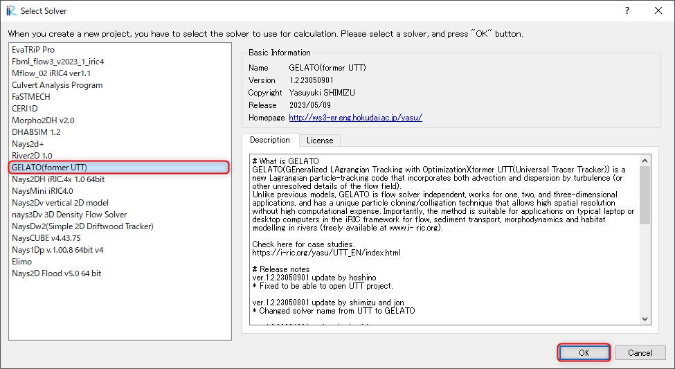
Figure 192 :Select GELATO Solve

Import Grid Data

Right click [Grid(No Data)] in the [Object Browser] and select [Import] as Figure 193.

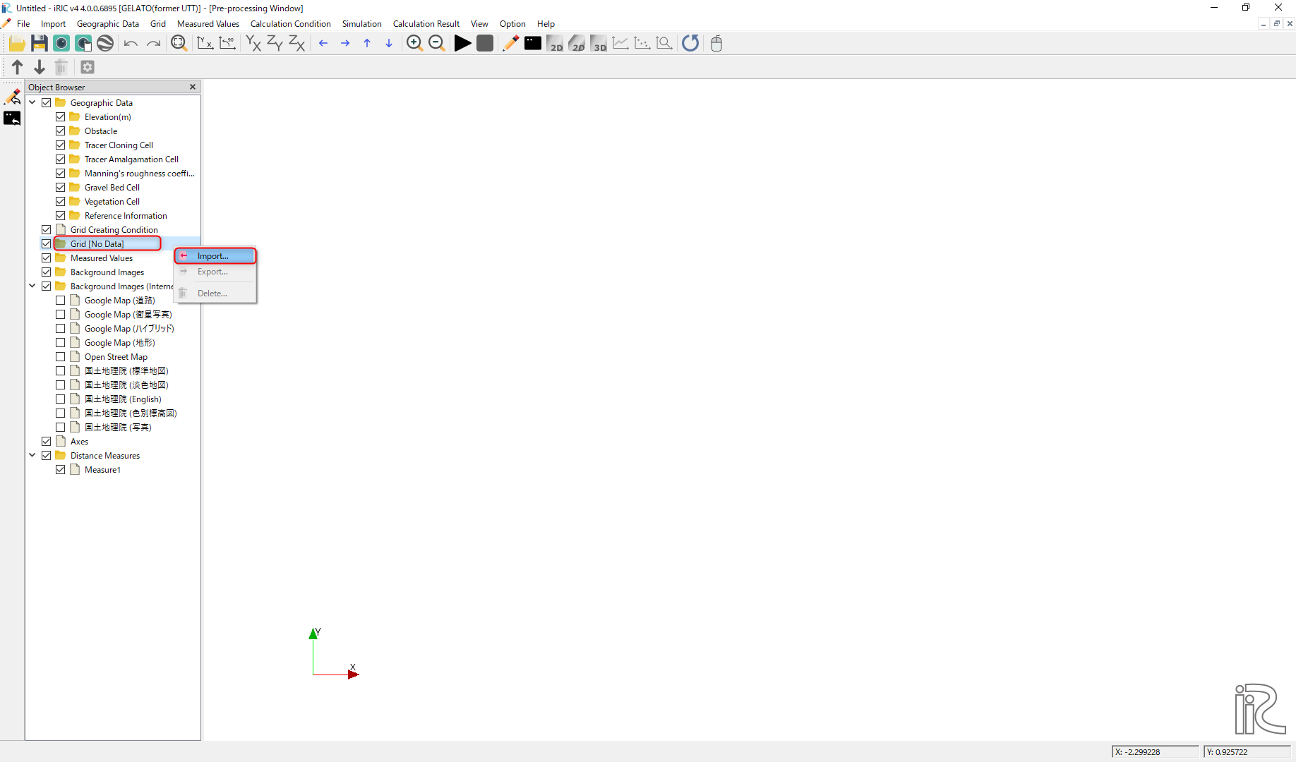
Figure 193 :Select GELATO

Choose [Case1.cgn] which contains the calculation results of [Nays2d+] saved in the previous section (Figure 194)

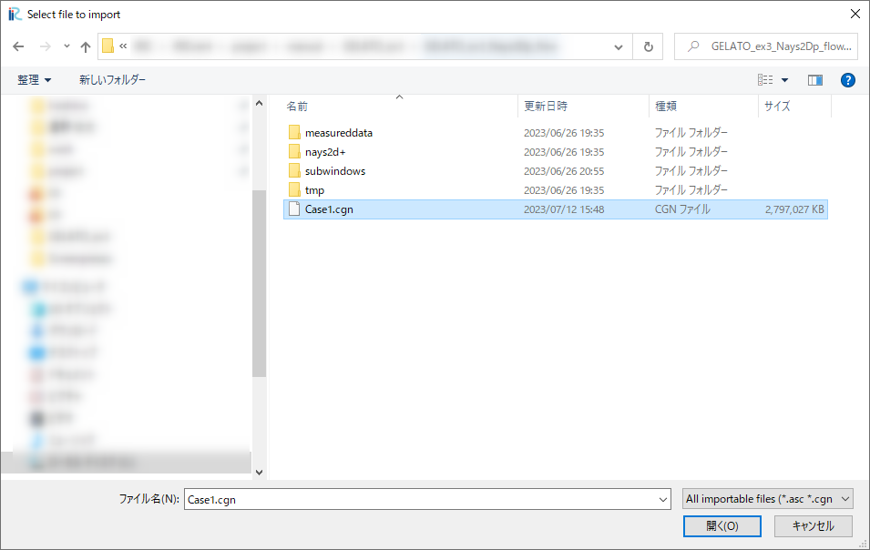
Figure 194 : Select a File to Import

Confirmation of Geographic Data

Set coordinate system by selecting [File]->[Property] from the main menu as Figure 195.

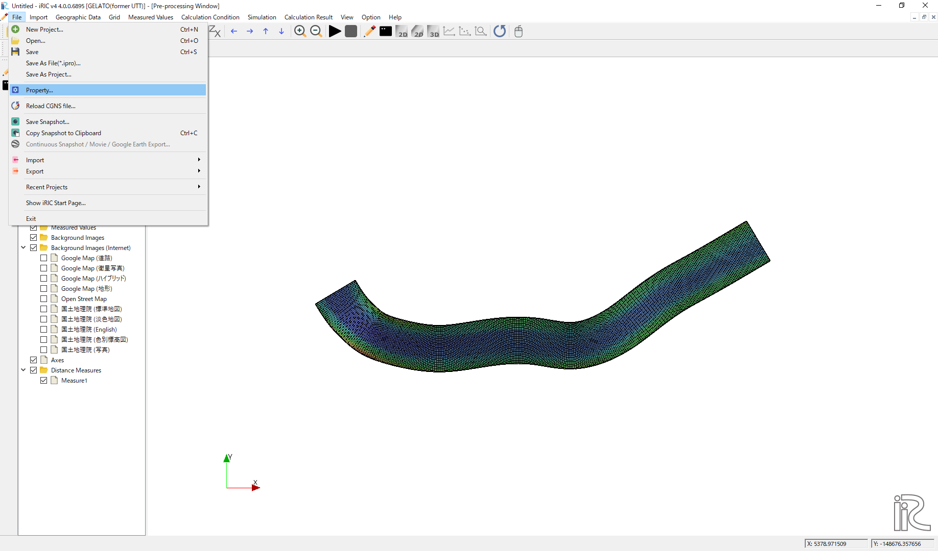
Figure 195 :Select Property

In the [Project Property] window, press [Edit] located at the [Coordinate System:] lin (Figure 196)

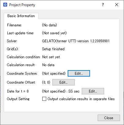
Figure 196 :Project Property

Type “Japan” in the box next to [Search:], select a line with [ EPSG:…Japan….CS VI], and press [OK] as Figure 197.

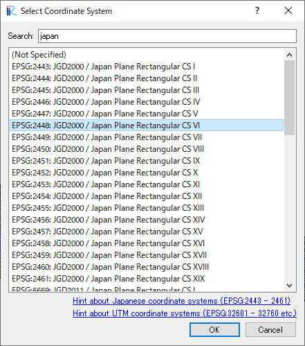
Figure 197 :Select Coordinate System

Select [Background Images(Internet)]->[国土地理院(標準地図)] from the Object Browser as Figure 198.

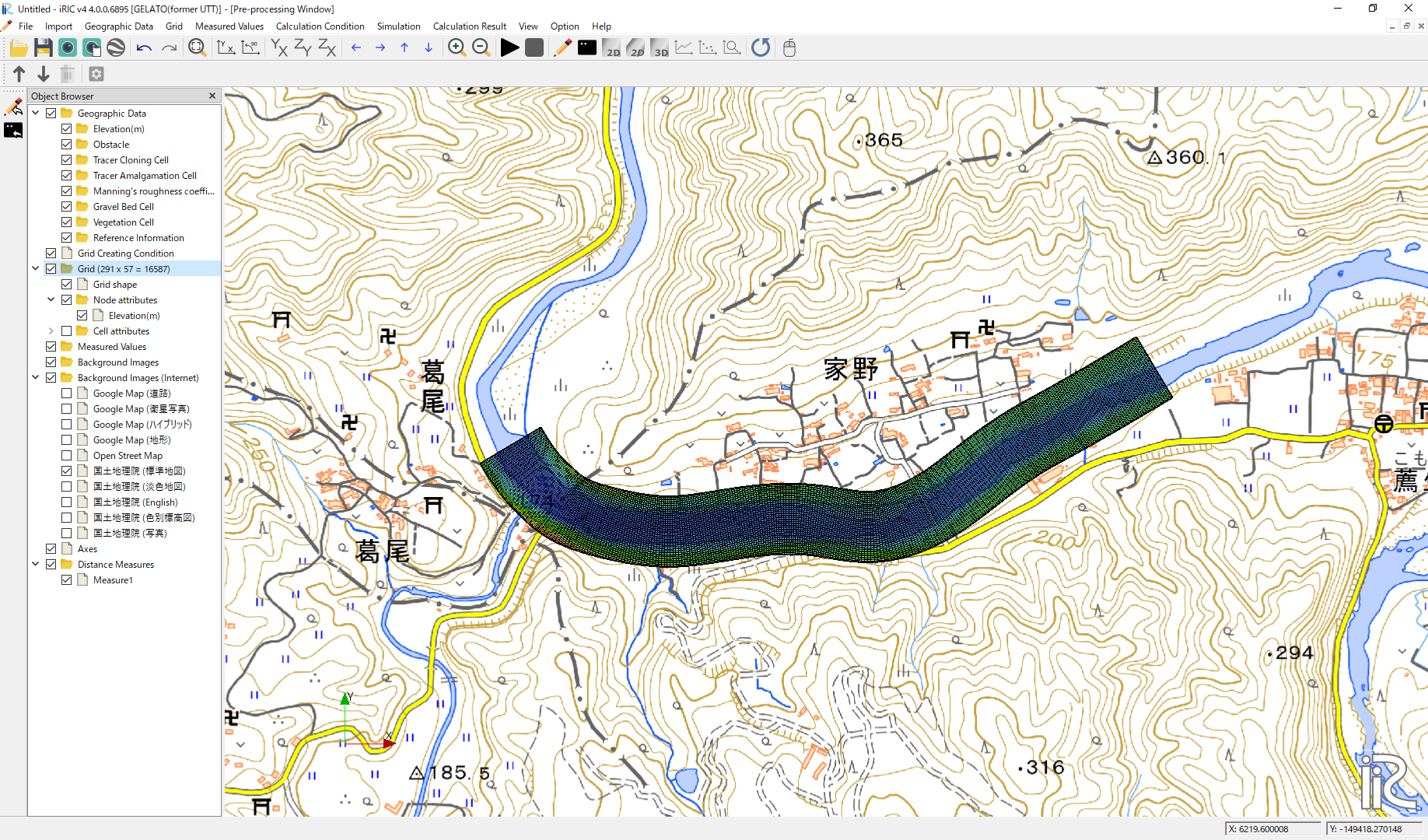
Figure 198 :Background Image

Tracer Tracking by GELATO

Calculation Condition

From the main menu, select [Calculation Condition]->[Setting], and set the [Calculation Condition] as Figure 199, Figure 200, Figure 201 and Figure 202. In which the CGNS file to read in the Figure 200 is usually the same file imported for calculation grid in Figure 194.

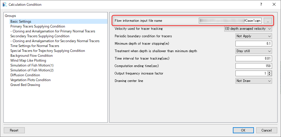
Figure 199 :[Basic Settings]

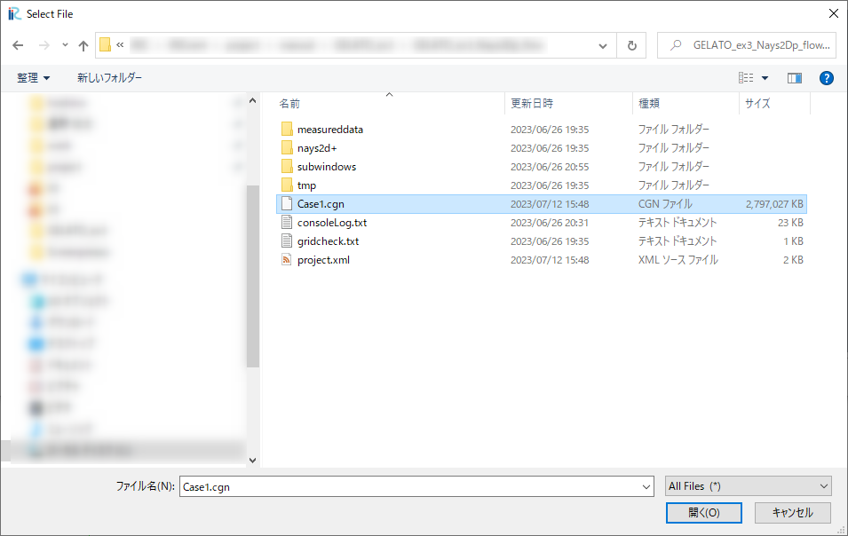
Figure 200 :Set the CGNS file to read the flow field information

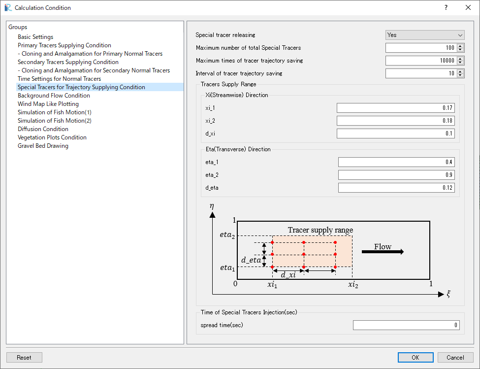
Figure 201 :Set special tracer information for path tracking

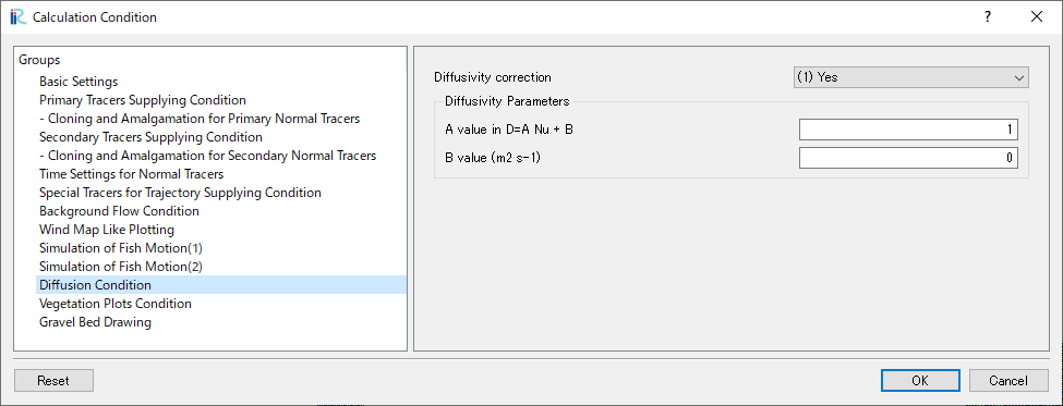
Figure 202 :Diffusion Condition

Execute Calculation

From the main menu, save thr project by selecting [File]->[Save Project as], and execute GELATO by selecting [Simulation]->[Run].

Visualization of the Calculation Results

From the main menu, select [Calculation Result]->[Open new 2D Post-Processing Window]. Put check marks in [Background Images(Internet)] and [国土地理院(標準地図)] in the Object Browser, as Figure 203.

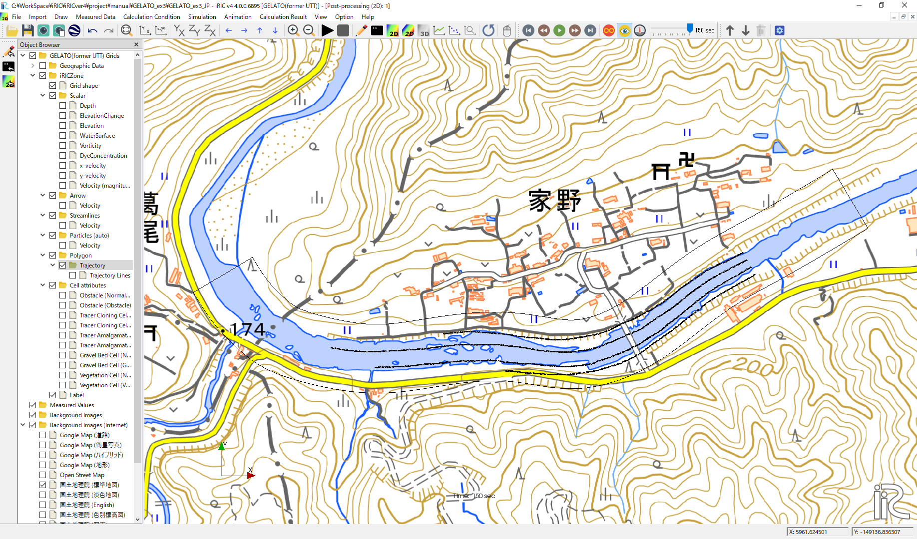
Figure 203 :Show Background Image

Right click the [Trajectory] at the [Polygon] in the Object Browser, and select [Property] as Figure 204.

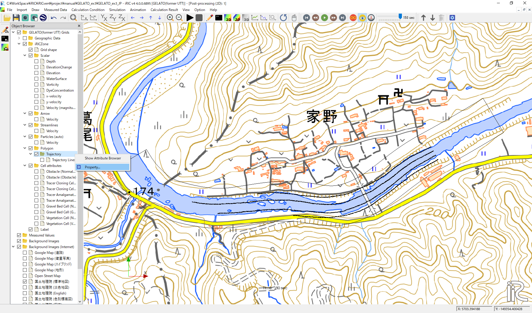
Figure 204 :Property of the Polygon

In the [Polygon Setting] window, set [Line Width] as [3] as Figure 205.

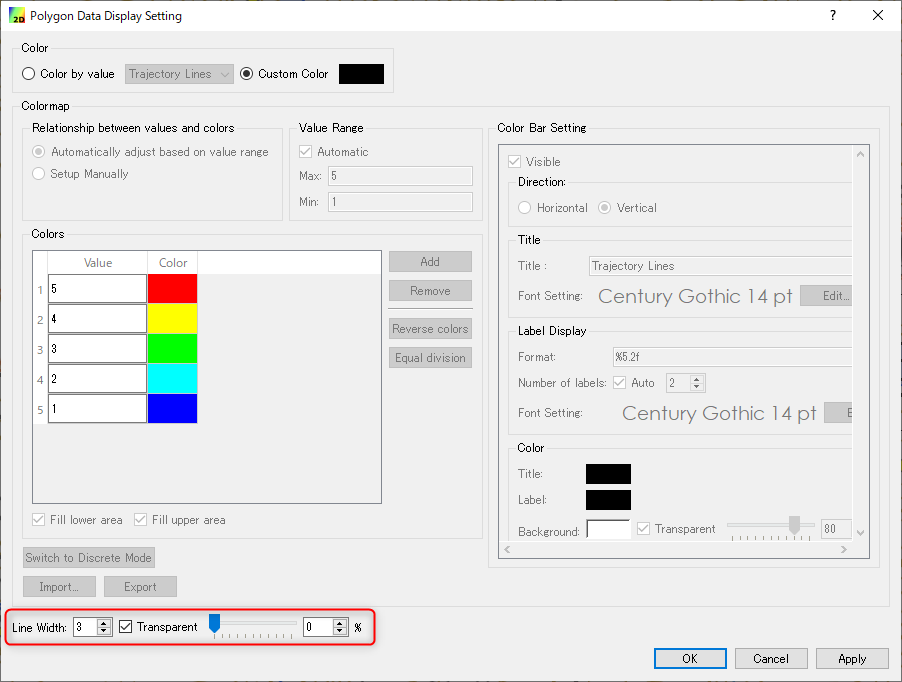
Figure 205 :Polygon Setting

From the Object Browser, put check marks at [Scalar(node)] and [Velocity] and right click [Velocity] and press [Property]. In the [Scalar Setting] window, as shown Figure 206, uncheck [Automatic], set [Max:] and [Min:] vales, and uncheck [Fill lower area].

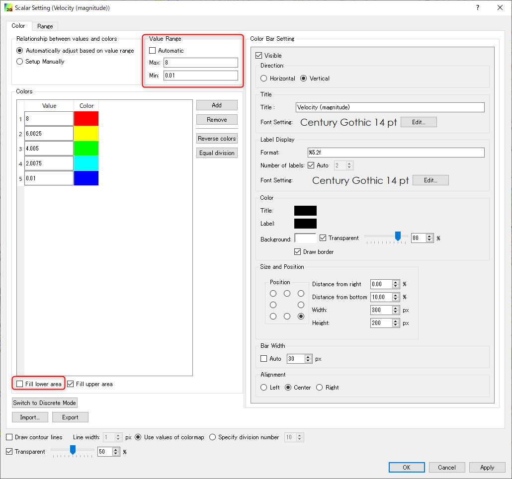
Figure 206 :Scalar Setting

After above settings the calculation results of the tracers injected from the Bridge can be visualized as follows.

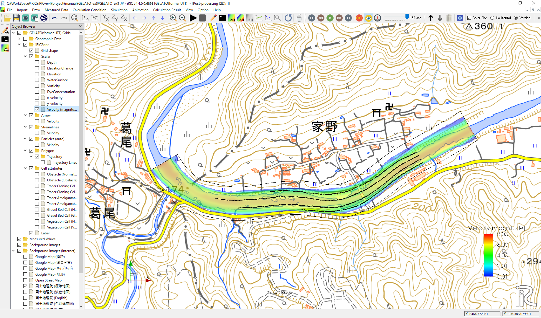
Figure 207 :Tracer Tracking Paths

Figure 208 : Tracer Tracking Animation